Talk with our engineers by joining the new Onehouse community Slack!
TL;DR
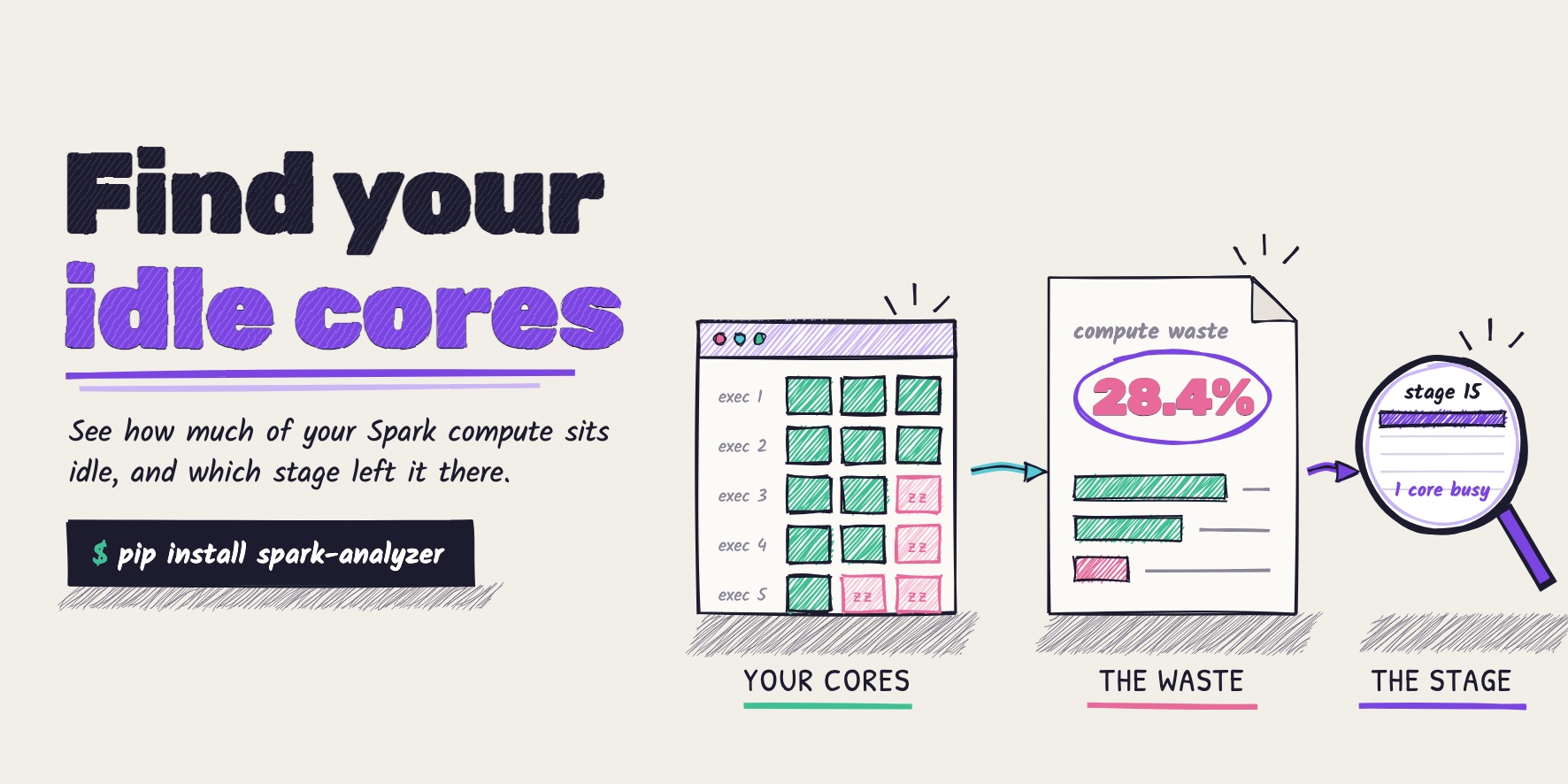
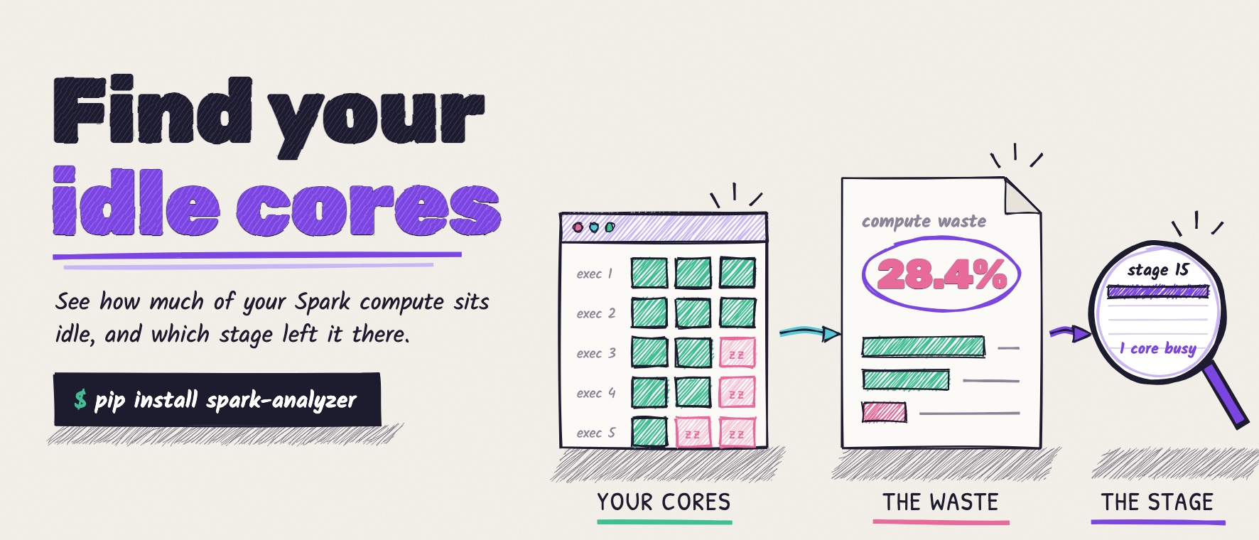
Cost Analyzer for Apache Spark™ (pip install spark-analyzer) is a free Python tool you run on your own machine. It reads the Spark History Server you already have, so nothing is installed on your cluster. In local-only mode, nothing leaves your environment. On a real nightly job with five executors of three cores each, the report showed 28.4% compute waste: about four of the fifteen cores did nothing for the whole run. Most of it came from one stage, a one-file CSV export where one core worked and fourteen waited.
Spark Analyzer: See how much of your Spark compute sits idle
When you submit an Apache Spark™ job, you set how many executors it gets and how many cores each one has. You pay for those cores from the moment the executors start until the job ends, whether tasks run on them or not. Most teams never find out how much of that time the cores sat idle.
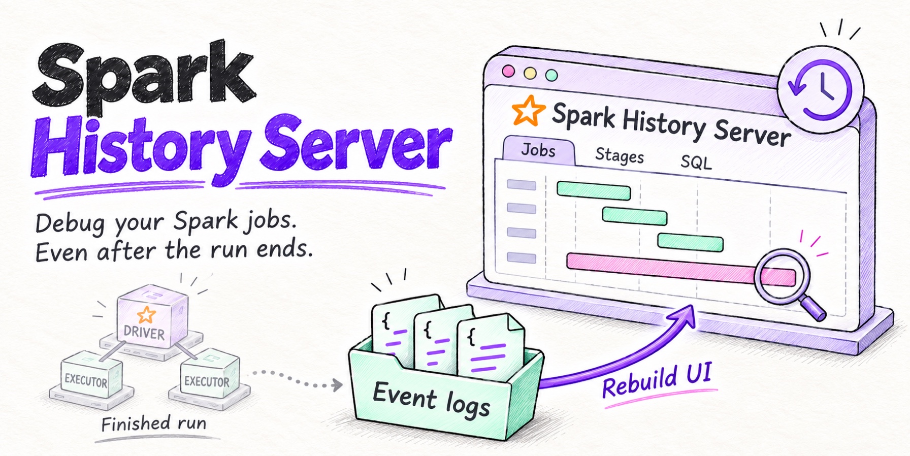
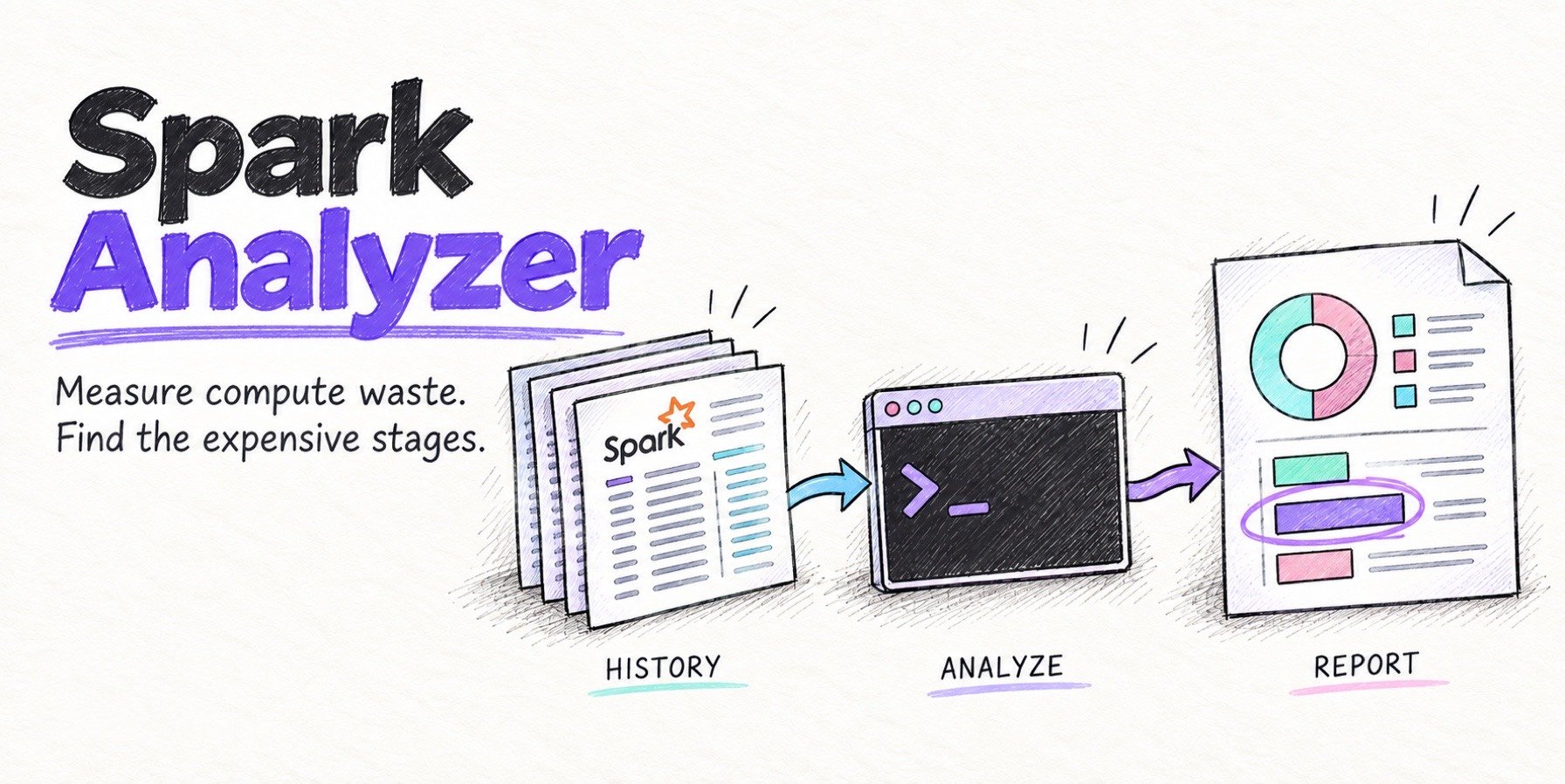
Cost Analyzer for Apache Spark measures it. It’s a free Python tool that you run on your own machine. It reads the Spark History Server you already have, and turns each run into a spreadsheet: how much compute the job reserved, how much it used, and which stages left cores waiting. Below, we run it on a real nightly job, from pip install to the stage that wasted most of the compute.
The problem: you pay for cores, not for work
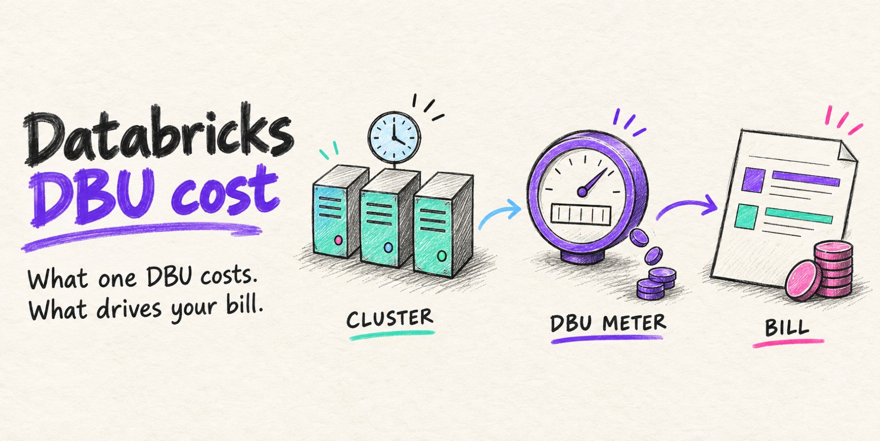
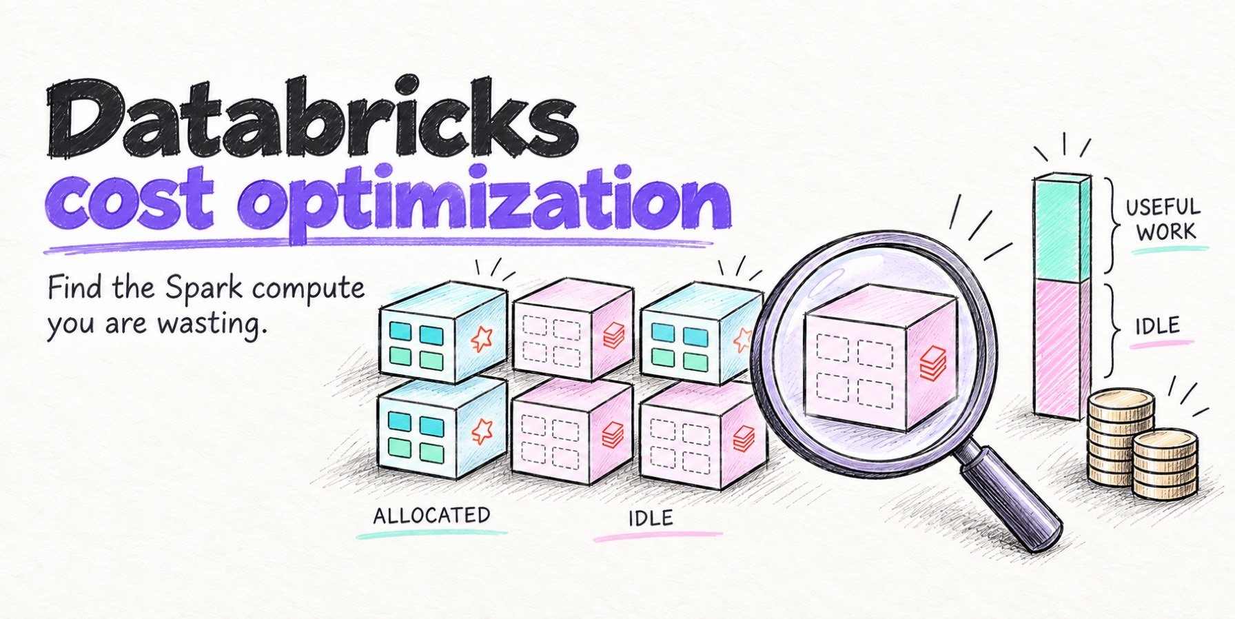
An executor holds its cores from the moment it starts until the job ends. Tasks use those cores only part of that time. The gaps, cores held but running nothing, are compute you pay for and don’t use.
The Spark UI doesn’t add this up for you. It lists every stage and every task, and it’s great for debugging a single run. But it never tells you how much of the compute you paid for sat idle, and one run of a modest job can have eighteen stages. Most teams run dozens of jobs a night.
The result
We ran Cost Analyzer on last night’s run of a real job, nightly_orders_etl. It read the History Server in a few seconds and produced one spreadsheet:
| Item | Result |
|---|---|
| The job | 5 executors × 3 cores = 15 cores, dynamic allocation off |
| Application duration | 4.37 minutes, 18 stages |
| Compute minutes used | 38.74 |
| Resource efficiency | 71.6% |
| Compute waste | 28.4%: about four of the fifteen cores idle for the whole run |
| Where the waste is | stage 15, a one-file CSV export: one core worked for 55 seconds while fourteen waited, about 12.9 of the 15.4 idle core-minutes |
| Installed on the cluster | nothing |
| Data sent anywhere | nothing, in local-only mode |
The example job
Our example job runs every night. It reads the last sixty days of orders from object storage (one folder of Parquet per day, about 200 MB each, roughly 12 GB in all), joins them with a customers table of two million rows, and totals revenue per customer and per region. It also writes yesterday’s orders as one CSV file for the finance team.
It runs as plain Apache Spark on a fixed cluster of six machines with four vCPUs each, one for the driver and five for the executors. The Spark configs ask for five executors with three cores each, with dynamic allocation off, so all fifteen cores are held for the whole run.
In the Spark History Server, last night’s run shows twelve jobs in about four and a half minutes. The Executors tab shows fifteen cores, 783 tasks and 35 minutes of task time. It doesn’t tell you how much reserved time went unused.
Install in seconds
You need Python 3, a terminal, and the address of your Spark History Server. The tool is on PyPI as spark-analyzer; we used version 0.1.38.
Create a virtual environment so the tool and its libraries stay apart from the rest of your Python, then install it:
# Create and activate a virtual environment
python3 -m venv .venv
source .venv/bin/activate

# Install the package
pip install spark-analyzer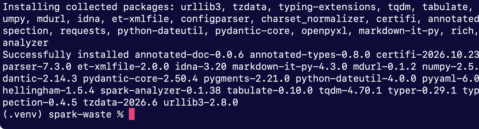
Run spark-analyzer --help to check if it worked. We use three of its commands: configure, analyze and report.
# Check the install and list the commands
spark-analyzer --help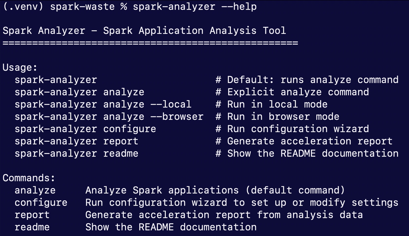
Connect it to your Spark History Server
Find the address
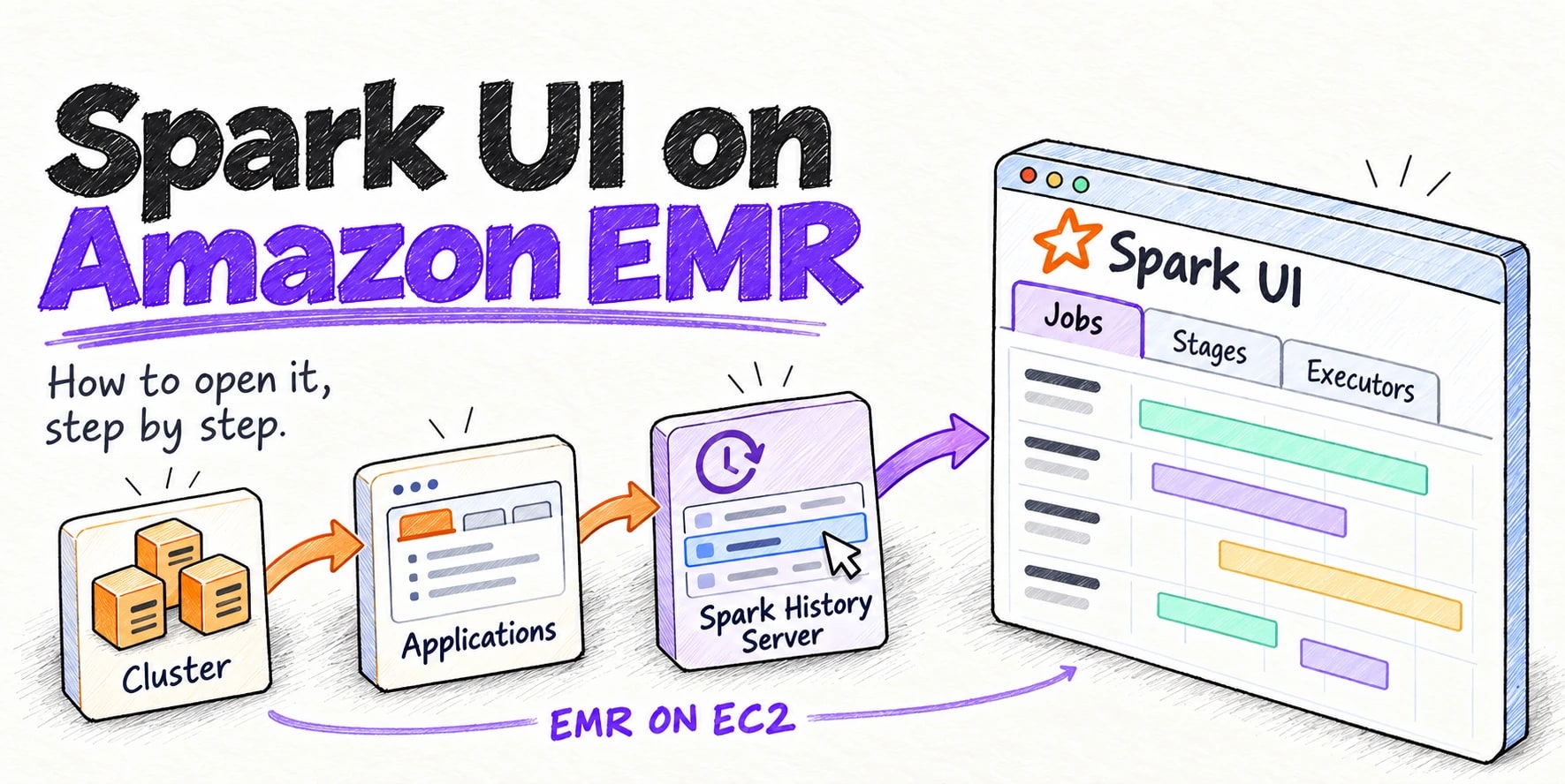
If you run Apache Spark yourself, the History Server is usually on port 18080. On a managed service such as Amazon EMR or Dataproc, forward that port to the machine you’re working on, or open an SSH tunnel, and you’ll reach it on localhost. You can also point the tool at a running application on port 4040.
Two modes: local-only or enhanced
The tool runs in one of two modes:
- Local-only mode needs no sign-up. You run the analysis with
--save-local, and the report is built where you run it. Nothing is sent anywhere. - Enhanced mode needs an ID from Onehouse. With an ID, the tool sends the stage metrics it collected to Onehouse over HTTPS, and you get a fuller report by email, with cost estimates. If your stage names are sensitive,
--opt-outturns them into hashes before anything is sent.
To get an ID, fill in the short form at onehouse.ai/spark-analysis-tool (name, job title, company and work email) and paste the ID when the tool asks for it. This walkthrough uses local-only mode.

Two ways to connect: local mode or browser mode
- Local mode talks to the History Server directly: on your own Apache Spark, through a port forward or SSH tunnel, or to a running application.
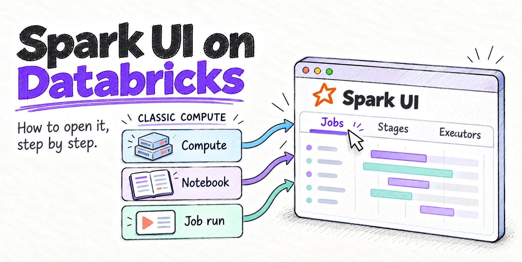
- Browser mode is for History Servers behind a web login, such as the Amazon EMR console or Databricks. It asks for your browser’s session cookie when it runs, and doesn’t save it.
Run the wizard
# Run the configuration wizard
spark-analyzer configure
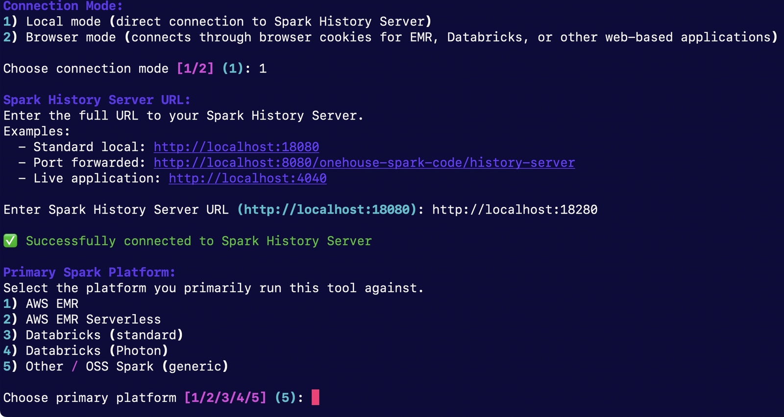
The first question is the optional ID; press Enter to skip it for local-only mode. Then choose local mode, paste the History Server address, and pick the platform you run on. The platform only changes the estimate at the end of the report.
Analyze a run
Run the analysis with --save-local:
# Complete local analysis: nothing is uploaded anywhere
spark-analyzer analyze --save-local
It lists the applications on your History Server and asks which to analyze. Paste the ID of the run you want; to analyze several runs, separate the IDs with commas. For each stage it reads the same details you see in the Spark UI: the steps inside the stage, how many tasks ran and for how long, and how much data went in and out. It also reads the executors, so it knows how long each one held its cores.
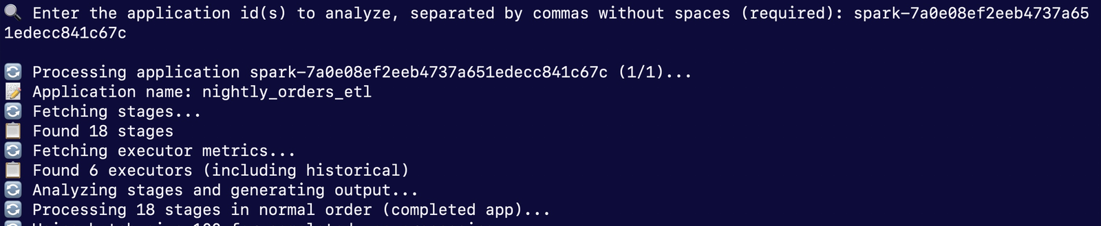
Each stage goes into one of three buckets: extract reads data in, transform works on it, and load writes it out. Stage 4 of our job reads the orders files and passes them on, so it counts as extract.
If you plan to share the report and your stage names show table names or file paths, add --opt-out with the fields to hash:
# Hash stage names, descriptions and details before you share the report
spark-analyzer analyze --save-local --opt-out name,description,details
Here is the same stage name in a plain run and in an --opt-out run:

The analysis is saved as a JSON file in spark_analysis_output/. One more command turns it into a spreadsheet:
# Turn the saved analysis into a spreadsheet
spark-analyzer report --input spark_analysis_output/*.json --output nightly_orders_etl.xlsx
Read the report
The spreadsheet has three tabs: App Level Summary, Workflow Level Summary and Stage Level Details.
The answer: compute waste
Start with the App Level Summary:
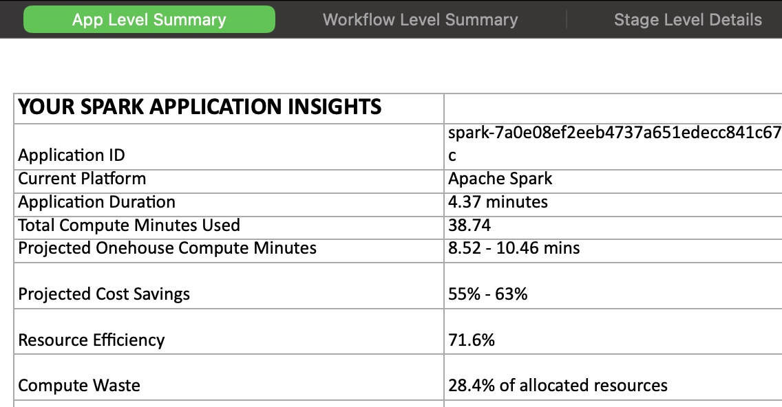
- Application duration is the wall-clock time: 4.37 minutes.
- Compute minutes used is the time tasks actually ran on cores, added up across all cores: 38.74.
- Resource efficiency is the share of the reserved core time that did work: 71.6%.
- Compute waste is the rest: 28.4%. On fifteen cores, that’s about four cores doing nothing for the whole run.
Under the summary, the report shows where the time goes. Stage 4, reading and joining sixty days of orders, runs the longest and does most of the work.
The workflow tab
The Workflow Level Summary groups the stages by bucket:
| Workflow type | Stages | Compute minutes | Workflow percentage |
|---|---|---|---|
| Extract | 6 | 35.37 | 78.02% |
| Transform | 1 | 2.25 | 5.29% |
| Load | 3 | 1.09 | 16.04% |
The report puts the other eight stages under “unknown”. Six of them were skipped and never ran, and together they used 0.02 compute minutes, so they don’t change the picture.
Six extract stages did almost all of the compute. The three load stages used about one compute minute between them, yet load takes 16% of the breakdown. Almost all of that is one stage, as the stage tab shows.
Finding the waste: duration vs compute minutes
The Stage Level Details tab has one row per stage. Compare each stage’s duration with its compute minutes. Dividing one by the other gives the average number of cores that were busy. These are the three longest stages; the other fifteen ran under six seconds each:
| Stage | Workflow type | Duration (min) | Compute minutes | Cores busy, on average (of 15) |
|---|---|---|---|---|
| 4 | Extract | 2.28 | 34.13 | 15.0 |
| 15 | Load | 0.92 | 0.92 | 1.0 |
| 6 | Transform | 0.19 | 2.25 | 11.7 |
- Stage 4 ran 2.28 minutes and used 34.13 compute minutes, so all fifteen cores were busy.
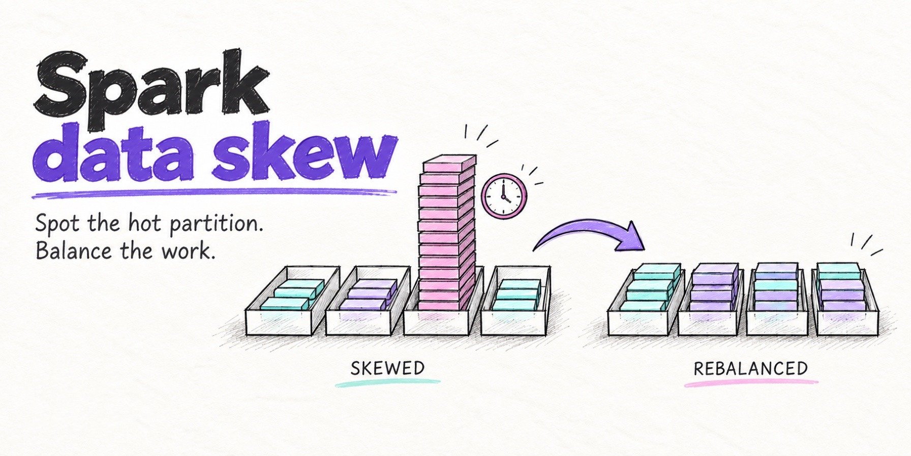
- Stage 15 ran 0.92 minutes and used 0.92 compute minutes. One core worked, and fourteen waited.
When compute minutes are close to duration times the number of cores, the stage used the cluster. When they’re close to the duration itself, one task ran and the rest of the cores waited.
Confirm it in the Spark UI
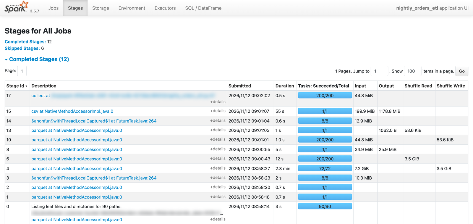
Open the Stages tab for the same run in the Spark History Server. Stage 15 stands out: one task (1/1), 55 seconds, 199.9 MiB in and 1178.8 MiB out. Stage 4, the big read, ran 72 tasks:
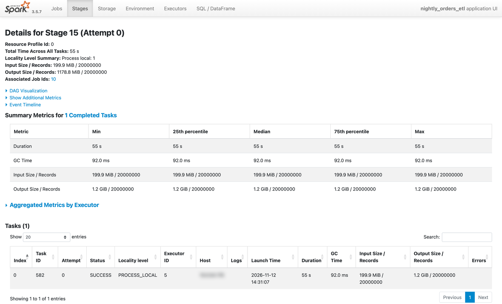
Stage 15’s detail page shows the cause. There is one task, so the minimum, median and maximum are all the same 55 seconds, and it ran on a single executor:
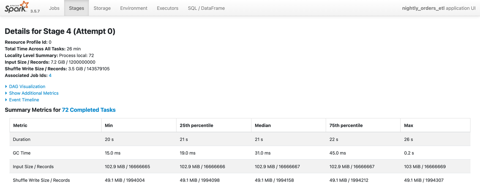
Compare stage 4. Its 72 tasks each ran 20 to 26 seconds on evenly split input, spread across all five executors, so every core had work:
The DAG for stage 15 shows what that one task did: it reads yesterday’s orders, coalesces them into a single partition, and writes one CSV file of twenty million rows:
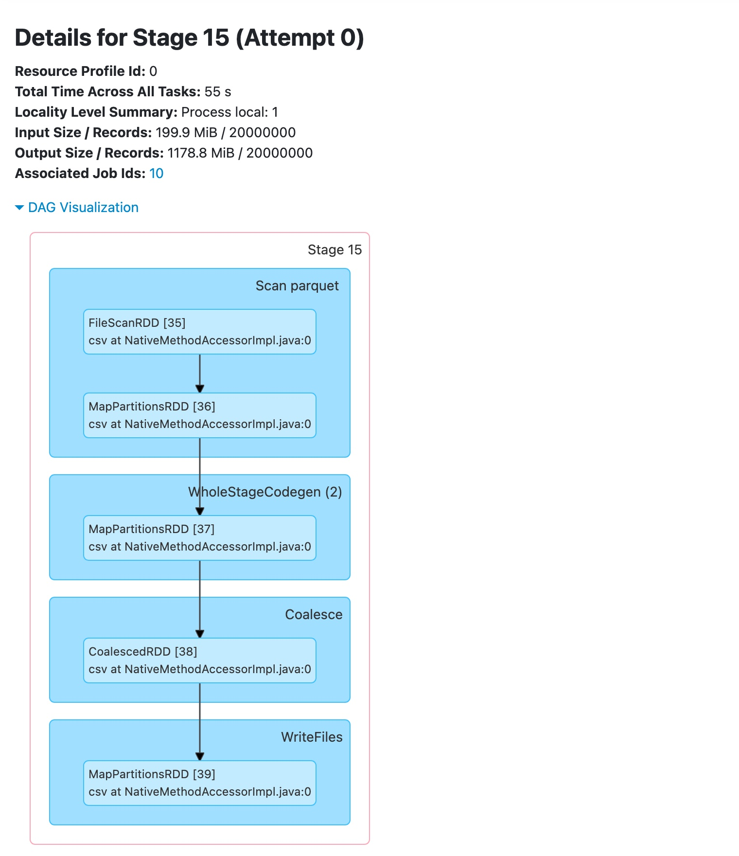
Fourteen cores held for 55 seconds with nothing to run is about 12.9 core-minutes, most of the job’s 15.4 idle core-minutes.
What to change
The report’s recommendations are a starting point: review resource allocation, and size executors and cores to what the job really uses. For this job, the stage tab already shows where to start:
- Write the export as several files instead of one, so more than one core does the work.
- Or move the export into its own small job with one or two cores, so the main job doesn’t hold fifteen cores while one works.
Then analyze the next run and compare. To compare jobs, analyze several runs at once and turn all the files into reports with one report command. Start with the job that has the highest waste.
One caution from our runs: cold starts move the number. When new nodes had to start and pull the Spark image, executors joined late and the same job showed a different waste figure. Compare runs that started the same way.
The Quanton estimate
The report also estimates the same job on Quanton, the Onehouse engine for Apache Spark, with no code changes. For this run it projects 8.52 to 10.46 compute minutes instead of 38.74, which is 73% to 78% fewer, and 55% to 63% lower cost:
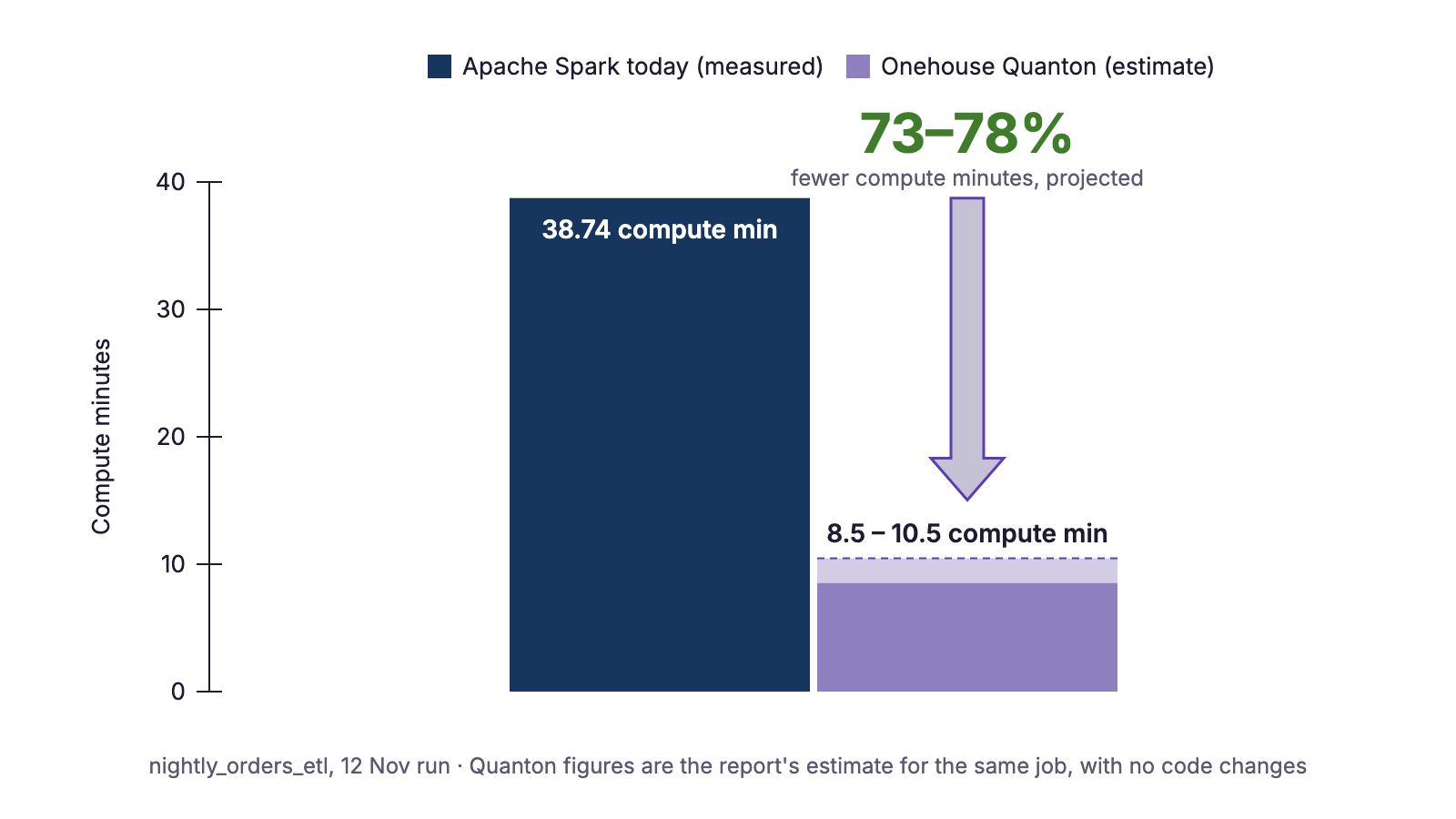
That’s an estimate. The idle compute above is measured from your own run. The estimates tend to be conservative: on one customer’s production workload migrated from Amazon EMR, Cost Analyzer predicted 27% acceleration, and the job went from 33 to 18 minutes on Quanton, 43.7% faster.
Conclusion
Cost Analyzer for Apache Spark turns a run you already have in the Spark History Server into one number: how much of the compute you reserved sat idle. On our nightly job it was 28.4%, about four of fifteen cores, and the stage tab showed the cause: a one-file export that kept fourteen cores waiting. In local-only mode, none of it leaves your environment.
Other recommended blogs:
- Meet Cost Analyzer – a free tool to unearth Apache Spark™ bottlenecks
- Spark Analyzer: Measuring Wasted Executor Time in Spark Jobs
Try the tool yourself with pip install spark-analyzer (PyPI), or reach out to Onehouse at gtm@onehouse.ai to work out how to optimize your Spark jobs and save on idle cores.
Frequently asked questions
Is it free?
Yes. pip install spark-analyzer and run it.
Does it install anything on my cluster?
No. It runs on your machine and reads the Spark History Server over HTTP. There’s nothing to deploy and no change request for your cluster.
Is my data shared with Onehouse?
Not in local-only mode. With --save-local and no ID, the analysis and the report stay on your machine, and none of it is shared with Onehouse or any external service. Only enhanced mode, with an ID, sends stage metrics to Onehouse, and --opt-out hashes the stage names first.
Which platforms does it work with?
Any Apache Spark with a Spark History Server: your own Apache Spark, Amazon EMR, EMR Serverless, Dataproc and Databricks. Use local mode for a History Server you can reach directly or through a tunnel, and browser mode for one behind a web login.
What’s the difference between compute minutes and duration?
Duration is wall-clock time. Compute minutes add up the time tasks ran on every core. A stage that keeps fifteen cores busy for one minute uses fifteen compute minutes; a stage that keeps one core busy for one minute uses one.
Can I analyze a running application?
Yes. Point it at the application’s Spark UI, usually on port 4040.
Can I analyze many jobs at once?
Yes. Paste several application IDs, separated by commas, and pass all the output files to spark-analyzer report.