Talk with our engineers by joining the new Onehouse community Slack!
TL;DR
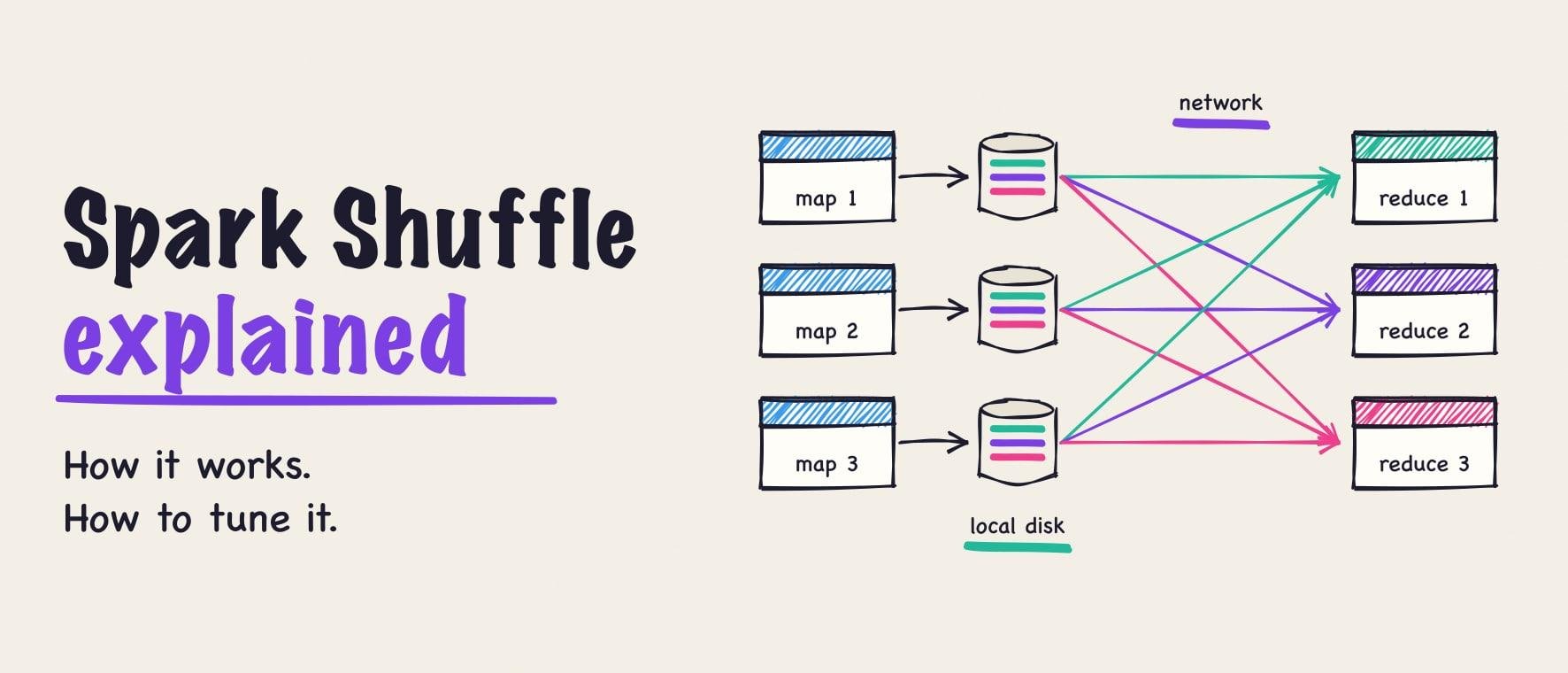
A Spark shuffle redistributes data across executors so that rows with the same key land in the same partition. Joins, aggregations, distinct, sorts, window functions and repartition all trigger one. Each shuffle splits the job into stages, writes map output to local disk, and pulls it back over the network, which makes it the most expensive step in most Spark jobs. Tune it in three moves: shuffle less data (filter early, broadcast small tables, reuse the table layout), size shuffle partitions to roughly 100 to 200 MB each instead of keeping the default of 200, and let adaptive query execution coalesce partitions and split skew at runtime.
A Spark shuffle is the step where Apache Spark™ moves data between executors so that every row with the same key ends up in the same partition. Spark needs it whenever one row’s result depends on rows that live on other machines: a join, a GROUP BY, a DISTINCT, a global sort, or a window function.
It is also, in most jobs, the most expensive thing Spark does. A shuffle writes data to local disk, sends it across the network, and reads it back, and it is where spill, skew, and fetch failures tend to show up. This guide builds the mental model first, then turns it into the checks and settings that make shuffles cheaper.
What a Spark shuffle is
Spark splits a dataset into partitions and processes each partition independently. That works for row-by-row operations such as filter or withColumn, because every output row depends only on one input row in the same partition.
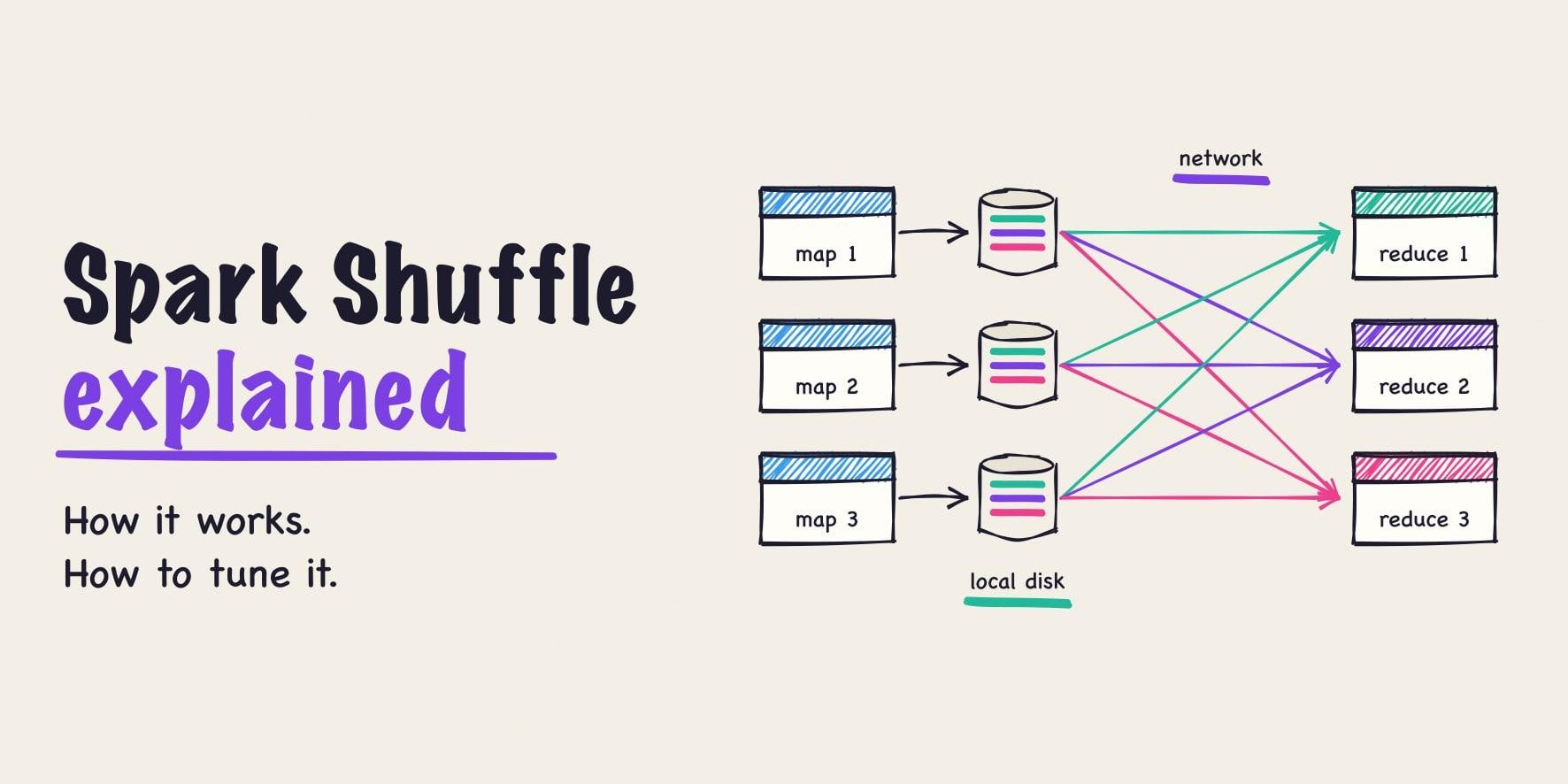
An aggregation breaks that assumption. To count orders per customer, all of a customer’s orders have to be in one place, but they start out spread across every partition of the input. The shuffle fixes this by hashing each row’s key, writing each row into the bucket for its target partition, and letting the next stage read each bucket from every executor that produced one.
Because a shuffle needs all of its input written before any of its output can be read, it is also where Spark draws a stage boundary. Everything before the shuffle runs as one stage, and everything after runs as the next.
What triggers a shuffle in Spark
Spark’s transformations fall into two groups. Narrow transformations compute each output partition from a single input partition, so they never move data. Wide transformations need rows from many input partitions, so they shuffle.
| Operation | Shuffles? | What you see in the plan |
|---|---|---|
filter, select, withColumn, union |
No | Filter, Project, Union |
coalesce(n) (fewer partitions) |
No | Coalesce |
groupBy().agg(), distinct, dropDuplicates |
Yes | Exchange hashpartitioning |
join on two large tables |
Yes, on both sides | Exchange hashpartitioning under SortMergeJoin |
join with a small table under the broadcast threshold |
No for the large side | BroadcastExchange + BroadcastHashJoin |
orderBy / sort (global) |
Yes | Exchange rangepartitioning |
Window.partitionBy(...) |
Yes | Exchange hashpartitioning under Window |
repartition(n) / repartition(col) |
Yes | Exchange RoundRobinPartitioning / hashpartitioning |
Two operations on that list avoid most of the cost. A broadcast join copies the small table to every executor instead of shuffling the large one. Aggregations do a partial aggregate on the map side before the exchange, so only one partial result per key and partition crosses the network. In the RDD API, this is the difference between reduceByKey, which combines on the map side, and groupByKey, which ships every value.
You can see the exchange in any DataFrame’s physical plan:
from pyspark.sql import SparkSession, functions as F

spark = SparkSession.builder.getOrCreate()
orders = spark.range(0, 10_000_000).withColumn(
    "customer_id", F.col("id") % 100_000
)

# Narrow: no shuffle
recent = orders.filter(F.col("id") > 9_000_000)

# Wide: rows must be regrouped by customer_id
per_customer = orders.groupBy("customer_id").count()
per_customer.explain()
== Physical Plan ==
AdaptiveSparkPlan isFinalPlan=false
+- HashAggregate(keys=[customer_id#2L], functions=[count(1)])
+- Exchange hashpartitioning(customer_id#2L, 200), ENSURE_REQUIREMENTS
+- HashAggregate(keys=[customer_id#2L], functions=[partial_count(1)])
+- Project [(id#0L % 100000) AS customer_id#2L]
+- Range (0, 10000000, step=1, splits=8)The Exchange node is the shuffle, and the 200 inside it is the number of shuffle partitions. The partial_count below it is the map-side partial aggregate. (Output trimmed: attribute IDs vary from run to run, and recent Spark versions also print a plan_id on each exchange.)
How a Spark shuffle works under the hood
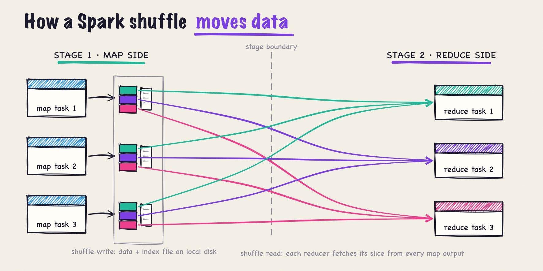
Since Spark 2.0, Spark’s built-in shuffle has been sort-based (the older hash-based shuffle was removed), and plugins that replace the shuffle manager follow the same overall shape. It has two halves: the map side, which writes shuffle files, and the reduce side, which fetches them.
The map side: shuffle write
Each task in the upstream stage computes its rows, assigns each row to a target partition with the partitioner (a hash of the key for joins and aggregations, key ranges for sorts), and writes them out grouped by partition. The result is one data file per map task, plus an index file that records where each partition’s block starts and ends. Both files go to the executor’s local disk, in the directories set by spark.local.dir or the cluster manager’s equivalent.
Spark picks one of three writers for each shuffle. When there is no map-side aggregation and few output partitions (at most spark.shuffle.sort.bypassMergeThreshold, 200 by default), it writes one file per partition and concatenates them. When rows can be sorted in serialized form, it uses the Tungsten serialized-sort writer, which avoids deserializing rows to sort them. Otherwise it sorts rows in memory, spilling sorted runs to disk when execution memory runs out, and merges the runs at the end.
The reduce side: shuffle read
When the downstream stage starts, each reduce task asks the driver’s MapOutputTracker where its partition’s blocks live, then fetches them through the BlockManager. Blocks on the same executor are read straight from disk, and remote blocks are pulled over the network, at most spark.reducer.maxSizeInFlight (48 MB by default) in flight at a time. The task then aggregates, joins, or sorts what it fetched, and can spill to disk again if it does not fit in memory.
The external shuffle service
Shuffle files belong to the executor that wrote them, so if that executor exits, its output disappears. The external shuffle service fixes this on YARN and standalone clusters. A long-running process on each node serves shuffle files on behalf of executors, so dynamic allocation can remove idle executors without losing their output. It is off by default (spark.shuffle.service.enabled=false) and must be installed on the nodes. Kubernetes has no equivalent service, which is covered in the section on elastic clusters below.
Why shuffles are expensive
Every shuffled byte is paid for several times. It is serialized and compressed on the map side, written to local disk, read back, sent over the network, decompressed and deserialized on the reduce side, and often spilled and read again if the reduce task runs out of memory. A shuffle-heavy stage spends its time on disk I/O, network transfer, and serialization CPU rather than on the computation the query asked for.
When a shuffle is too large for the cluster, it tends to fail in a few recognizable ways:
No space left on device: shuffle files or spill filled the executor’s local disks.FetchFailedExceptionorMetadataFetchFailedException: Missing an output location for shuffle: a reduce task could not fetch a block, usually because the executor that wrote it died or was removed. Spark then reruns the map stage that produced it, which can turn into a long chain of stage retries.OutOfMemoryErroror a container killed by the cluster manager: a reduce task received a partition much larger than its memory, often because of skew or too few partitions.
Spark shuffle partitions
The setting that decides how many partitions a DataFrame shuffle produces is spark.sql.shuffle.partitions. Its default is 200, and it applies to every join and aggregation in Spark SQL and the DataFrame API, whether the shuffle moves 2 GB or 2 TB.
It is easy to confuse with spark.default.parallelism, which serves a similar purpose for the RDD API. spark.default.parallelism sets the default partition count for RDD shuffles such as reduceByKey and for parallelize. When it is unset, RDD shuffles use the largest parent RDD’s partition count and parallelize uses the total number of executor cores. It does not set the partition count of DataFrame or SQL shuffles.
Both directions of a wrong value cost something:
| Too few shuffle partitions | Too many shuffle partitions |
|---|---|
| Each task gets gigabytes of data | Each task gets a few megabytes |
| Spill to disk, long GC pauses, OOM kills | Scheduling overhead dominates task time |
| Few tasks, so idle cores on a large cluster | Many tiny shuffle blocks and fetch requests |
| One slow task holds up the whole stage | Thousands of small output files on write |
On Databricks, spark.sql.shuffle.partitions also accepts auto, which lets the platform pick the count. That value is Databricks-only. Open-source Apache Spark expects a number, and gets similar behavior from adaptive query execution, covered next.
How to size shuffle partitions, and let AQE help
A practical starting point is to aim for shuffle partitions of roughly 100 to 200 MB each, measured by the stage’s Shuffle Write size in the Spark UI, and to round the count to a multiple of the cluster’s total cores so tasks run in even waves.
Here is a worked example. A daily job shuffles 300 GB in its largest stage on a cluster of 50 executors with 4 cores each, or 200 task slots.
- With the default of 200 partitions, each task reads about 1.5 GB. Most of that spills, and the stage runs as one long wave.
- 300 GB divided by a 200 MB target is about 1,536 partitions. Rounding to 1,600 gives 8 even waves across 200 slots, with each task reading about 190 MB.
You rarely have to hand-tune every query, though. Adaptive query execution (AQE), on by default since Spark 3.2, re-plans a query at each shuffle boundary using the actual sizes of the shuffle output. Three of its features target shuffles directly:
- Partition coalescing. AQE merges small adjacent shuffle partitions toward
spark.sql.adaptive.advisoryPartitionSizeInBytes(64 MB by default). It means a high initial partition count does not leave you with thousands of tiny tasks. - Skew join handling. A partition larger than 5 times the median and larger than 256 MB is split into smaller tasks, with the matching rows on the other side of the join replicated to each.
- Join strategy changes. If one side of a sort-merge join turns out to be small at runtime, AQE switches it to a broadcast hash join and reads the shuffle locally.
A common pattern is to set a deliberately high initial partition count and let AQE coalesce downward:
--conf spark.sql.adaptive.enabled=true \
--conf spark.sql.adaptive.coalescePartitions.enabled=true \
--conf spark.sql.adaptive.coalescePartitions.initialPartitionNum=2000 \
--conf spark.sql.adaptive.advisoryPartitionSizeInBytes=128m \
--conf spark.sql.adaptive.coalescePartitions.parallelismFirst=false \
--conf spark.sql.adaptive.skewJoin.enabled=true
The parallelismFirst line matters more than it looks. With parallelismFirst at its default of true, AQE ignores the advisory size and coalesces only as far as the cluster’s default parallelism allows. That favors many small tasks, and the Spark performance tuning guide recommends setting it to false on a busy cluster. Defaults above match the current Apache Spark documentation; check them against your Spark version.
How to spot shuffle problems
The plan tells you where shuffles happen, and the Spark UI tells you how much each one cost. Use both.
In the query plan
Run explain() (or EXPLAIN FORMATTED in SQL) and look for these nodes:
Exchange hashpartitioning(key, N): a shuffle by key, withNpartitions.Exchange rangepartitioning: a global sort, which also runs a sampling job to pick ranges.BroadcastExchange: a broadcast instead of a shuffle on that side of the join.AQEShuffleRead coalescedorskewed: in the final plan after the query runs, AQE merged or split the shuffle partitions.
Two exchanges in a row with nothing in between, or an exchange directly above a repartition you added yourself, usually means the data is shuffled twice.
In the Spark UI
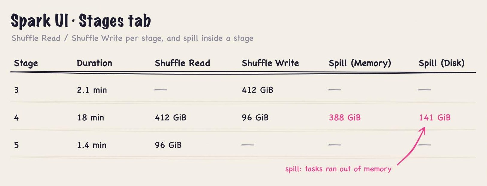
The Stages tab carries the numbers. For each stage, Shuffle Write is the data written for the next stage, and Shuffle Read is the data fetched from the previous one. Open a stage and two more columns matter. Spill (Memory) is the size of spilled data while it was in memory, and Spill (Disk) is its size once serialized to disk. Any nonzero spill means tasks did not have enough memory for their share of the shuffle.
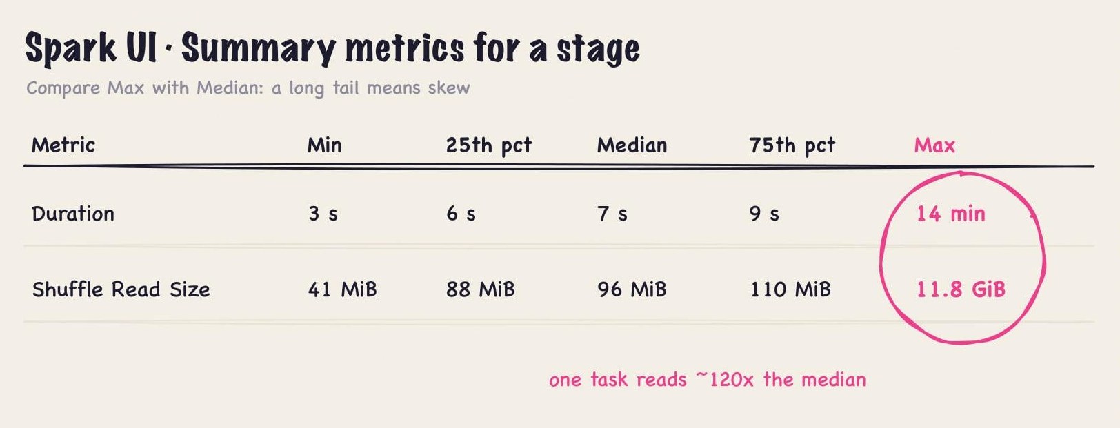
Skew shows up in the stage’s summary metrics table. Compare the Max column with the Median for Duration and Shuffle Read Size. If the slowest task reads ten times what the median task reads, a few keys hold a large share of the data, and adding partitions will not help, because every row for one key still goes to one partition.
For a walkthrough of reading stages, task metrics, and SQL plans end to end, the recording of the Onehouse Deep Dive session Read the Spark UI Like a Profiler covers the same signals on a real job.
How to reduce Spark shuffle cost
Partition sizing makes a shuffle run better. The bigger wins usually come from shuffling less data in the first place.
Filter and project before wide operations. Spark pushes filters toward the scan where it can, but a filter after a join, or a select * carried into a groupBy, still ships columns and rows the result does not need. Every column you drop before an exchange shrinks the shuffle.
Broadcast small tables. A table under spark.sql.autoBroadcastJoinThreshold (10 MB by default) is broadcast automatically. For a dimension table that is larger but still fits comfortably in executor memory, use a hint such as /*+ BROADCAST(dim) */ or F.broadcast(dim), or raise the threshold. The shuffle hash join vs. sort-merge join post covers what each join strategy costs once a shuffle is unavoidable.
Aggregate before you join. If a join is followed by an aggregation on the larger side, aggregate first and join the smaller result.
Do not repartition without a reason. repartition(n) always shuffles. To reduce the number of output files, coalesce(n) merges partitions without a shuffle, and the REBALANCE hint lets AQE size output partitions for you.
Reuse the table layout. If two large tables are joined on the same key every day, store them bucketed on that key. Joins between bucketed Spark tables, and between compatible Apache Iceberg™ tables through storage-partitioned joins (spark.sql.sources.v2.bucketing.enabled), can skip the exchange entirely.
Fix skew at the key. AQE splits skewed join partitions automatically. For skewed aggregations, or skew AQE does not catch, salt the hot keys: add a random suffix, aggregate on the salted key, then aggregate again without it. The Spark data skew guide walks through detection and each fix.
Once the data volume is right, a few shuffle I/O settings are worth knowing:
| Setting | Default | What it does |
|---|---|---|
spark.shuffle.compress |
true |
Compresses map output. Leave it on. |
spark.io.compression.codec |
lz4 |
Codec for shuffle and spill. zstd trades CPU for smaller shuffles on network-bound jobs. |
spark.shuffle.file.buffer |
32k |
In-memory buffer per shuffle output stream. Raising it (for example to 1m) cuts disk writes and syscalls. |
spark.reducer.maxSizeInFlight |
48m |
Data each reduce task fetches at once. Raise it on fast networks with memory to spare. |
spark.local.dir |
/tmp |
Where shuffle and spill files go. Point it at fast local NVMe, not network storage. |
Shuffle on elastic and Kubernetes clusters
Autoscaling and shuffle work against each other. Dynamic allocation removes idle executors to save money, but an idle executor may still be holding shuffle output that a later stage needs. If it is removed, that output is lost and the stage that produced it reruns.
On YARN, the external shuffle service solves this. On Kubernetes, which has no external shuffle service, Spark offers two mechanisms, and some teams add a third:
- Shuffle tracking (
spark.dynamicAllocation.shuffleTracking.enabled, on by default in Spark 3.5 and 4.x) keeps executors alive while they hold shuffle data that active jobs still need. It is safe, but it can keep a scaled-up cluster at full size long after the work has moved on. - Graceful decommissioning (
spark.decommission.enabledwithspark.storage.decommission.enabled, since Spark 3.1) migrates an executor’s shuffle blocks to other executors before it is removed, which suits spot interruptions and scale-down. - Remote shuffle services such as Apache Celeborn™ store shuffle data outside the executors, so executors can come and go freely. They are a separate service to deploy and run.
Spark’s own push-based shuffle, which merges shuffle blocks on the server side, is supported only on YARN with the external shuffle service. The Spark dynamic allocation guide covers how these interact with autoscaling in more depth.
Where the execution engine fits
Everything above is query-level and configuration-level tuning, and it applies to any Spark deployment. The execution engine also decides how much a shuffle costs: how rows are encoded and compressed, how memory and spill are managed, and which operations need a full shuffle at all. No engine removes shuffles. A join on unpartitioned data still has to bring matching keys together.
Quanton is a drop-in Spark execution engine from Onehouse, and it can be used on its own without the Onehouse platform. Two of its features relate directly to this guide. Its low-shuffle MERGE for Apache Iceberg and Apache Hudi™ scales work with the change set instead of shuffling the whole target table. In Onehouse’s test on a 1 TB Iceberg table with about 5% of rows changed, it ran roughly 6x faster than open-source Spark (3.6 minutes against 21) and moved about 1 TB less shuffle data. Its AI Spark engineer, free on every plan, diagnoses bottlenecks such as skew and OOMs from the plan, metrics, and logs inside the Spark UI. Onehouse publishes its full engine comparisons on the Quanton benchmarks page, and you can try Quanton on your own jobs by creating an account.
A Spark shuffle checklist
- Find every
Exchangein the plan, and remove the ones you added yourself without a reason. - Cut the data before it crosses an exchange: filter, project, pre-aggregate, and broadcast small sides.
- Size
spark.sql.shuffle.partitionsfor roughly 100 to 200 MB per partition, or set a high initial count and let AQE coalesce. - Check Spill (Memory), Spill (Disk), and Max against Median task metrics in the Spark UI after every change.
- Treat skew as a key problem, not a partition-count problem: AQE skew joins first, salting where AQE does not reach.
- On autoscaling clusters, decide deliberately between shuffle tracking, decommissioning, and a remote shuffle service.
Frequently asked questions
What is a shuffle in Spark?
A shuffle is the redistribution of data across partitions and executors so that all rows with the same key end up in the same partition. Spark performs one for joins, aggregations, distinct, global sorts, window functions, and repartition. Each shuffle writes map output to local disk, transfers it over the network, and starts a new stage.
What is the default value of spark.sql.shuffle.partitions?
The default is 200 in open-source Apache Spark. It applies to joins and aggregations in Spark SQL and the DataFrame API. With adaptive query execution enabled, which is the default since Spark 3.2, Spark can coalesce those partitions at runtime based on the actual shuffle size.
Does coalesce cause a shuffle?
No. coalesce(n) reduces the number of partitions by merging existing ones on the same executors, without a shuffle. repartition(n) always shuffles, and so does coalesce(n, shuffle=True) in the RDD API. Coalescing to a very small number can leave a few large, slow tasks, because it does not rebalance the data.
What is shuffle spill in Spark?
Spill happens when a task’s shuffle data does not fit in its execution memory, so Spark writes sorted runs to disk and merges them later. The Spark UI reports it as Spill (Memory), the size while in memory, and Spill (Disk), the size once serialized. Spill usually means shuffle partitions are too large, the data is skewed, or executors have too little memory per core.
What is the difference between spark.sql.shuffle.partitions and spark.default.parallelism?
spark.sql.shuffle.partitions sets the number of partitions for DataFrame and SQL shuffles, with a default of 200. spark.default.parallelism sets the default partition count for RDD operations such as reduceByKey, join on RDDs, and parallelize. When it is unset, RDD shuffles use the largest parent RDD’s partition count and parallelize uses the total number of executor cores. Setting one does not change the shuffle partition count of the other API.
Is spark.sql.shuffle.partitions=auto available in open-source Spark?
No. The auto value is a Databricks feature. In open-source Apache Spark, set a number and enable adaptive query execution’s partition coalescing, which adjusts the effective partition count at runtime from the actual shuffle size.