Spark repartition vs coalesce: differences, shuffle cost, and when to use each

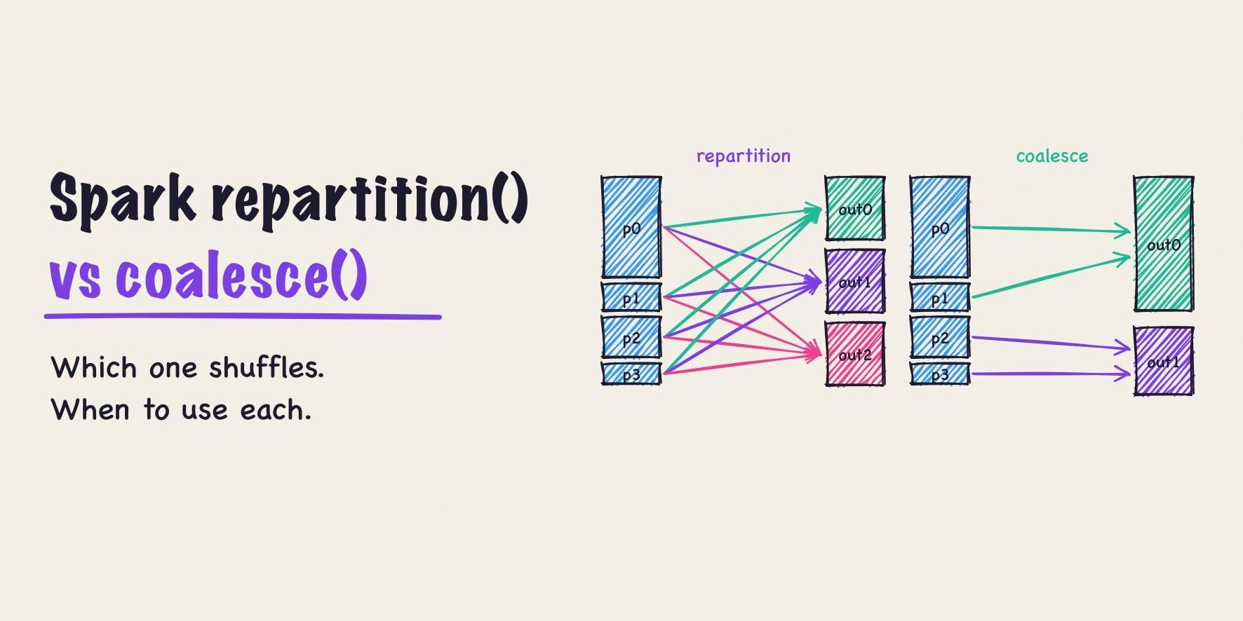
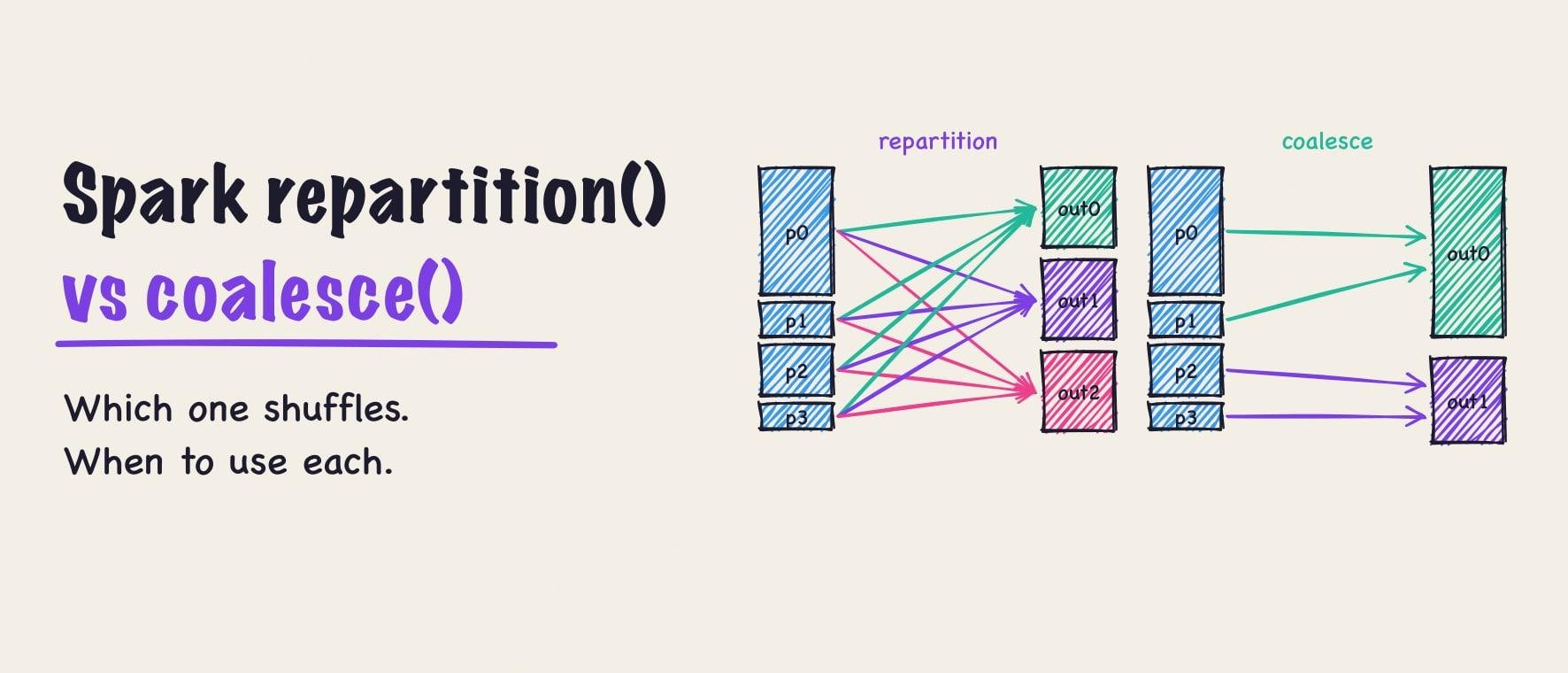
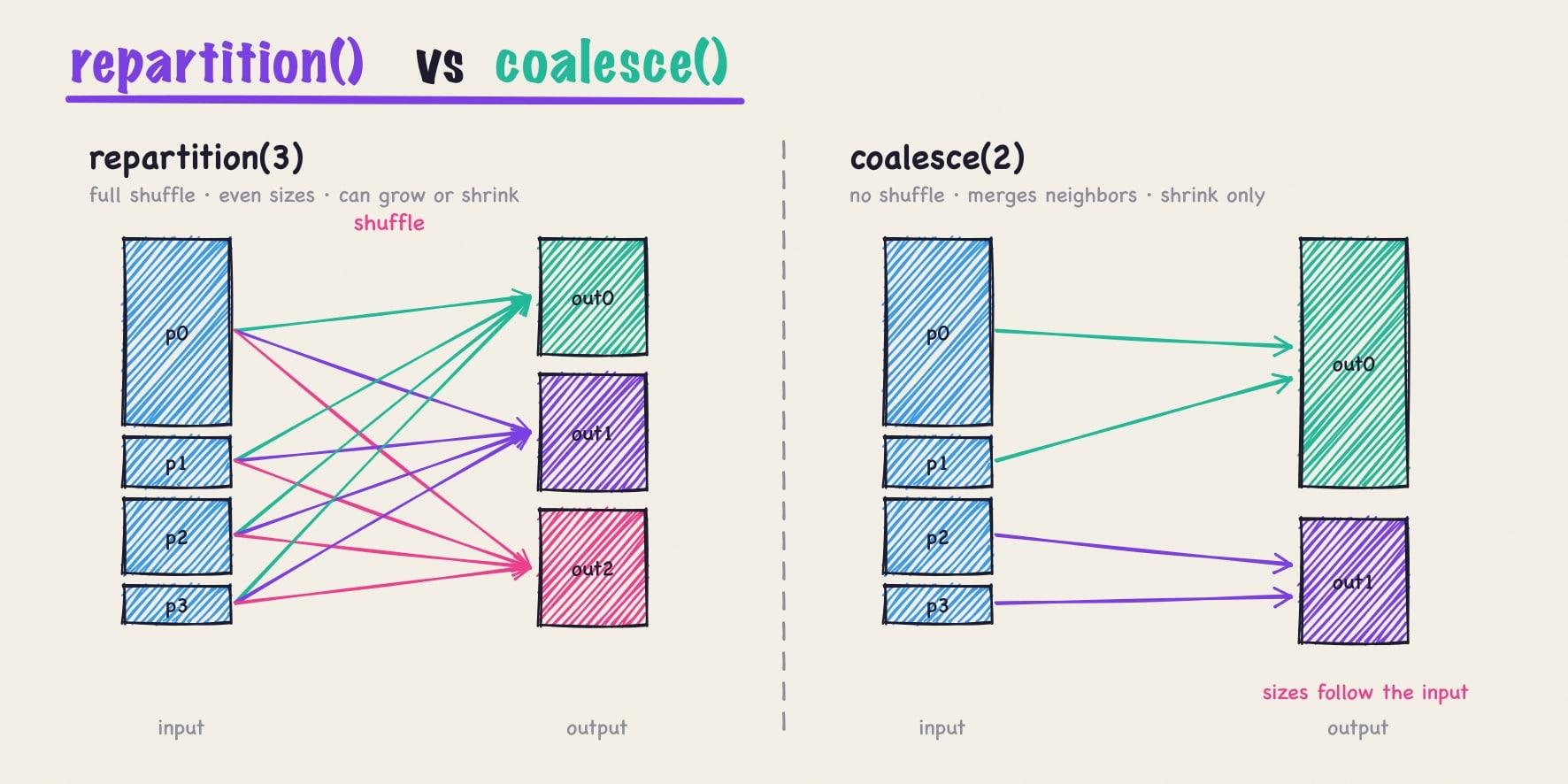
Spark repartition vs coalesce comes down to one trade-off. Both methods change how many partitions a DataFrame has. repartition() does it with a full shuffle, so it can raise or lower the count and spread rows evenly. coalesce() does it by merging partitions that already exist, so it skips the shuffle but can only lower the count, and it can leave the result unevenly sized.

Most of the time the choice is made right before a write, when a job is about to produce too many small files. This guide covers what each method does, which one shuffles, the case where coalesce() makes a job slower instead of faster, and how to pick between them.

Quick answer: repartition() vs coalesce()

Use repartition() to increase partitions, to fix uneven partition sizes, to group rows by a column, or to cut partitions sharply after expensive upstream work. Use coalesce() for a modest reduction on data that is already reasonably balanced, typically just before a write.

	repartition(n)	coalesce(n)
Shuffle	Yes, a full shuffle	No (on DataFrames)
Direction	Increase or decrease	Decrease only
Resulting partition sizes	Even (round-robin) or by key (hash)	Whatever the merged partitions add up to
Effect on upstream work	Upstream keeps its parallelism; a new stage starts after the shuffle	The whole stage runs with n tasks
New stage in the Spark UI	Yes	No
Typical use	Rebalancing, increasing parallelism, grouping by key, large reductions	Fewer output files from balanced data

What partitions control in Spark

A partition is the chunk of data that one task processes. The number of partitions in a stage is the most tasks that stage can run at once, so it sets how much of the cluster a stage can use.

The starting count depends on where the data comes from. A file scan splits input into partitions of up to spark.sql.files.maxPartitionBytes (128 MB by default). An RDD created with parallelize uses spark.default.parallelism. Any join or aggregation produces spark.sql.shuffle.partitions partitions, 200 by default, before adaptive query execution adjusts them.

You can check the current count at any point:

df.rdd.getNumPartitions()

# On Spark Connect, where df.rdd is not available:
from pyspark.sql import functions as F
df.select(F.spark_partition_id()).distinct().count()

How repartition() works

repartition() always runs a full shuffle. Every task in the current stage writes its rows into new buckets, and a new stage reads them back as the requested number of partitions. That is what lets it increase the count and even out partition sizes. It is also what makes it cost a shuffle’s worth of disk, network, and serialization.

It has three forms, and they distribute rows differently:

• repartition(n) deals rows out round-robin, so the n partitions come out close to equal in size.
• repartition(n, "col") or repartition("col") hashes the column, so all rows with the same value land in the same partition. This is what you want before a write partitioned by that column, but a skewed key stays skewed: one value with half the rows still makes one huge partition.
• repartitionByRange(n, "col") assigns contiguous value ranges to partitions, using a sample of the data to pick the boundaries, so the result can differ slightly between runs.

The partition count is exact in one case and adjustable in the other. repartition(n) and repartition(n, "col") produce exactly n partitions, and adaptive query execution (AQE) leaves that number alone. repartition("col") with no number starts from spark.sql.shuffle.partitions, and AQE can coalesce it to fewer partitions at runtime.

df = spark.range(0, 1_000_000, 1, 8)
df.repartition(4).explain()

== Physical Plan ==
AdaptiveSparkPlan isFinalPlan=false
+- Exchange RoundRobinPartitioning(4), REPARTITION_BY_NUM, [plan_id=7]
   +- Range (0, 1000000, step=1, splits=8)

The Exchange node is the shuffle. REPARTITION_BY_NUM records that you asked for a fixed number of partitions. (The plan_id varies from run to run.)

How coalesce() works

coalesce() is a narrow transformation. It does not redistribute rows the way a shuffle does. It groups existing partitions together, and each output task computes or reads its group of parent partitions one after another. Going from 1,000 partitions to 100, each new partition takes roughly 10 of the old ones.

Three consequences follow from that design:

• It can only reduce. On a DataFrame, asking for more partitions than you have leaves the count unchanged. df.coalesce(16) on an 8-partition DataFrame still has 8 partitions.
• It does not rebalance. Spark groups partitions by count and data locality, not by size. If the input partitions are uneven, the merged ones are too.
• It changes the stage it sits in. Because there is no shuffle boundary, the coalesce runs in the same stage as the work before it. That stage now runs with n tasks. The next sections show why that matters.

df = spark.range(0, 1_000_000, 1, 8)
df.coalesce(4).explain()
df.coalesce(16).rdd.getNumPartitions() # 8: coalesce cannot increase

== Physical Plan ==
Coalesce 4
+- *(1) Range (0, 1000000, step=1, splits=8)

There is no Exchange, and no AdaptiveSparkPlan wrapper either, because AQE only wraps plans that contain a shuffle or a subquery.

The RDD API is the exception to “coalesce never shuffles”. rdd.coalesce(n, shuffle=True) adds a shuffle step, can increase the count, and is what rdd.repartition(n) calls internally. The DataFrame coalesce() has no such option.

Repartition vs coalesce: which one shuffles?

Only repartition() shuffles. You can confirm it in two places.

In the plan, repartition() adds an Exchange node, and coalesce() adds a Coalesce node with no exchange below it.

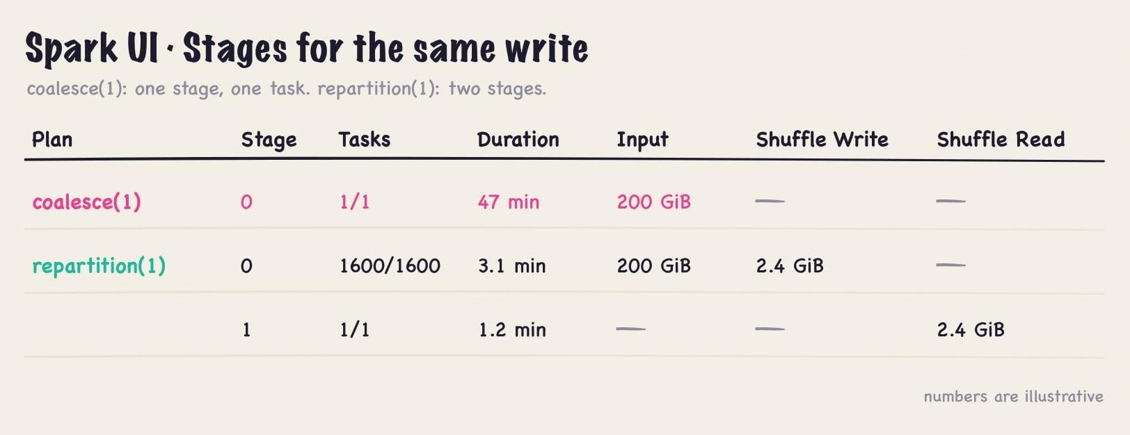
In the Spark UI, repartition() splits the job into one more stage. The stage before it shows Shuffle Write, and the new stage shows Shuffle Read of roughly the same size. With coalesce(), the stage count does not change; the existing stage simply runs fewer tasks.

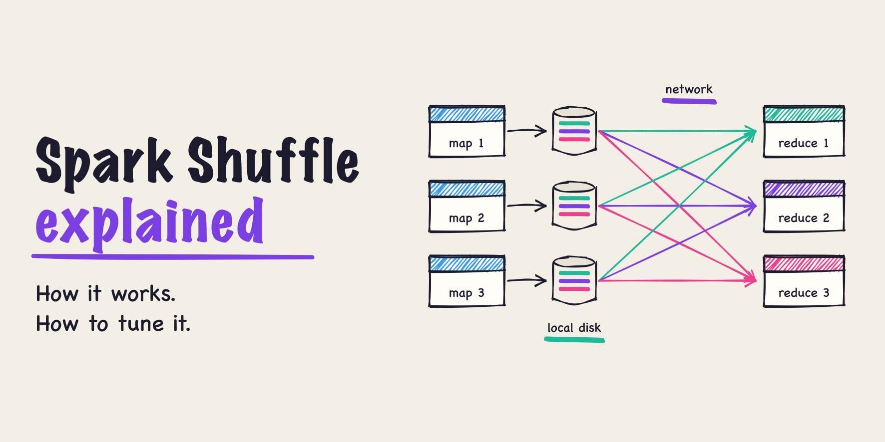
The shuffle is not free. Every row is serialized, written to local disk, sent over the network, and read back, and shuffles are where spill and fetch failures usually show up. Our companion guide, Spark shuffle, explained, covers what happens during a shuffle and how to size it. That cost is why coalesce() is the usual advice for reducing partitions, and why that advice has an important exception.

When coalesce() backfires

The common rule, “use coalesce to reduce partitions because it avoids a shuffle”, is right for modest reductions and wrong for drastic ones. Because coalesce(n) runs in the same stage as the operations before it, everything back to the previous shuffle boundary (or back to the scan) now runs with n tasks.

Consider a job that reads 200 GB, filters and transforms it, and writes one report file:

# Slow: the read, filter, and transform all run in ONE task
(spark.read.parquet("s3://bucket/events/")
    .filter(F.col("event_date") == "2026-10-01")
    .withColumn("revenue", F.col("price") * F.col("qty"))
    .coalesce(1)
    .write.mode("overwrite").parquet("s3://bucket/daily_report/"))

# Better: the scan and transforms run in parallel, then one task writes
(spark.read.parquet("s3://bucket/events/")
    .filter(F.col("event_date") == "2026-10-01")
    .withColumn("revenue", F.col("price") * F.col("qty"))
    .repartition(1)
    .write.mode("overwrite").parquet("s3://bucket/daily_report/"))

In the first version, the scan that would have run as about 1,600 tasks runs as one. The cluster sits idle while a single core reads, filters, and transforms everything. In the second version, the scan and the transforms keep full parallelism, the results are shuffled to one partition, and only the final write is single-threaded. Paying for the shuffle is far cheaper than giving up the parallelism.

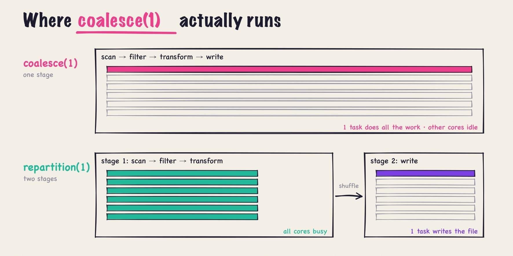
The PySpark coalesce() documentation gives the same advice for drastic reductions such as numPartitions = 1: call repartition(), which adds a shuffle but keeps the upstream partitions running in parallel.

The trap does not apply when a shuffle already sits right before the coalesce(). After a groupBy, for example, the coalesce() only narrows the post-aggregation stage, which is often small. In the Spark UI, check how many tasks the stage containing your coalesce() runs, and how long they take.

coalesce() also cannot fix skew. If one input partition is ten times the size of the others, the merged partition that contains it is still the largest. A round-robin repartition(n) evens out sizes. A hash repartition by a skewed column does not, and the Spark data skew guide covers the fixes for that case.

Controlling output files when writing

Each write task produces at least one file for each output directory it writes to. The number of partitions at the write is therefore the main lever on how many files you get and how large they are.

• Fewer files from balanced data: df.coalesce(n) before the write. It is the cheapest option when the stage is not doing heavy work and the partitions are similar in size.
• Fewer files after heavy work, or from uneven data: df.repartition(n). It costs a shuffle but produces evenly sized files and keeps upstream parallelism.
• One file: repartition(1) after heavy work, coalesce(1) only when the data is small and already cheap to compute. Either way, one task writes the whole output, so this only suits small results.

Partitioned writes need more care. With .write.partitionBy("event_date"), every task writes a file into every date directory it has rows for, so 200 tasks and 30 dates can produce up to 6,000 small files. Repartitioning by the same column first sends each date to one task:

(df.repartition("event_date")
    .write.partitionBy("event_date")
    .option("maxRecordsPerFile", 5_000_000)
    .parquet("s3://bucket/events_by_date/"))

Each date now gets one file, unless it has more than 5 million rows. maxRecordsPerFile (or spark.sql.files.maxRecordsPerFile, which defaults to 0 for no limit) splits a large date into several files, so a busy day does not turn into one oversized file.

Where AQE and SQL hints fit

Adaptive query execution has a feature called partition coalescing, and despite the name it is a different mechanism from coalesce(). With AQE on (the default since Spark 3.2), Spark merges small shuffle partitions after a shuffle, based on the actual data sizes, toward spark.sql.adaptive.advisoryPartitionSizeInBytes (64 MB by default). It applies to shuffles from joins and aggregations, and to repartition("col") without a number. It never changes repartition(n) or a coalesce() you wrote yourself.

In Spark SQL, the same controls are available as hints:

SELECT /*+ COALESCE(10) */ * FROM events;
SELECT /*+ REPARTITION(200, event_date) */ * FROM events;
SELECT /*+ REPARTITION_BY_RANGE(event_date) */ * FROM events;
SELECT /*+ REBALANCE(event_date) */ * FROM events;

REBALANCE is the one with no DataFrame method of its own (use df.hint("rebalance", "event_date")). It shuffles like a repartition but lets AQE pick the partition count and split skewed partitions toward the advisory size. That makes it a good default before a write when you want sensibly sized files and do not want to choose a number.

Repartition or coalesce: a decision guide

Situation	Use
Reduce partitions a little, data is balanced, little work in the stage	coalesce(n)
Reduce partitions sharply (for example to 1) after a heavy scan or transform	repartition(n)
Increase partitions to use more of the cluster	repartition(n)
Partition sizes are uneven	repartition(n) (round-robin) or the REBALANCE hint
Rows with the same key must end up together, for example before partitionBy	repartition("col") or repartition(n, "col")
Output should be split into sorted value ranges	repartitionByRange(n, "col")
You want Spark to size the partitions for you	AQE with repartition("col"), or REBALANCE

Whichever you choose, check the result in the Spark UI: the number of tasks in the stage that contains the change, whether a new stage appeared, and the Max against Median shuffle read size for the tasks after it.

Quanton’s free AI Spark engineer, built into the Spark UI, diagnoses bottlenecks such as skew from the plan, metrics, and logs, which is where a misplaced coalesce() shows up. Quanton is a separate Spark engine from Onehouse that can be used without the Onehouse platform, and you can try it by creating an account.

Frequently asked questions

Does coalesce cause a shuffle in Spark?

Not on a DataFrame. coalesce(n) merges existing partitions within the current stage, so no data is shuffled and no new stage is created. On an RDD, coalesce(n, shuffle=True) does add a shuffle and behaves like repartition(n).

Can coalesce increase the number of partitions?

No. On a DataFrame, coalesce() with a number larger than the current partition count leaves the count unchanged. Use repartition(n) to increase partitions.

Is repartition(1) better than coalesce(1)?

It depends on what runs before it. If the stage reads or transforms a lot of data, repartition(1) is usually much faster, because the upstream work keeps its parallelism and only the final step runs in one task. coalesce(1) is fine when the data is already small and cheap to produce.

Does repartition fix data skew?

repartition(n) with no columns spreads rows round-robin, so it evens out partition sizes. repartition("col") hashes the column, so every row with the same value lands in one partition, and a skewed key stays skewed. For skew in joins, AQE’s skew handling or salting the key is the usual fix.

What is the difference between repartition and repartitionByRange?

repartition() assigns rows by round-robin or by a hash of the columns, so related values are not kept in order. repartitionByRange() assigns contiguous ranges of the column’s values to each partition, which suits sorted output and range queries. It samples the data to choose the ranges, so boundaries can vary slightly between runs.

Is AQE partition coalescing the same as coalesce()?

No. AQE merges small partitions after a shuffle, automatically and based on actual sizes, and only for shuffles it is allowed to resize. coalesce() is an explicit, narrow merge that you place in the plan, and it changes the parallelism of the stage it runs in.