Talk with our engineers by joining the new Onehouse community Slack!
TL;DR
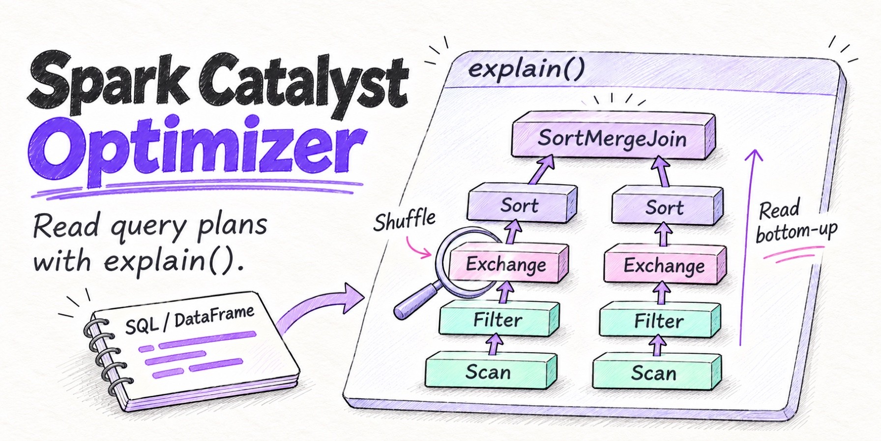
The Spark Catalyst optimizer turns SQL, DataFrame and Dataset code into one logical plan, rewrites it with rules such as predicate pushdown, column pruning and constant folding, then picks physical operators and inserts shuffles. explain() prints the result: simple shows the physical plan, extended adds the parsed, analyzed and optimized logical plans, cost adds size and row estimates, formatted numbers every operator, and codegen shows the generated Java. Read a physical plan from the bottom up, check PartitionFilters and PushedFilters on each scan, count the Exchange nodes, and confirm the join strategy. With adaptive query execution on, explain() shows the initial plan (isFinalPlan=false); the plan Spark actually ran is in the Spark UI SQL tab.
The Spark Catalyst optimizer is the query optimizer inside Spark SQL. It takes the SQL, DataFrame or Dataset code you write, turns it into a tree of logical operators, rewrites that tree with rules, and chooses the physical operators that Apache Spark™ runs on the cluster. explain() prints what Catalyst decided. Reading that output is the fastest way to find out why a job shuffles more data than you expected, skips a broadcast join, or reads every partition of a table.
This guide follows one query through each stage of Catalyst, then reads its plans line by line. Every plan below is real output from Spark 4.3.0 running locally (local[8], with spark.sql.shuffle.partitions set to 8). File paths are shortened, and ... marks trimmed lines.
What the Spark Catalyst optimizer is
Catalyst is an extensible optimizer built on trees and rules, described in the Spark SQL paper and Databricks’ deep dive. A query is a tree of operators, and a rule replaces a pattern in that tree with an equivalent, cheaper one. Spark applies batches of rules until the tree stops changing, and new optimizations such as dynamic partition pruning (Spark 3.0) arrived as new rules.
SQL, DataFrame and Dataset code all compile into the same logical plan representation, so they get the same optimizations. We wrote the example query below both ways, and after normalizing attribute IDs the two physical plans were identical. Catalyst can’t see inside a Python or Scala UDF, and RDD code bypasses it entirely.
The Catalyst pipeline: From query to physical plan
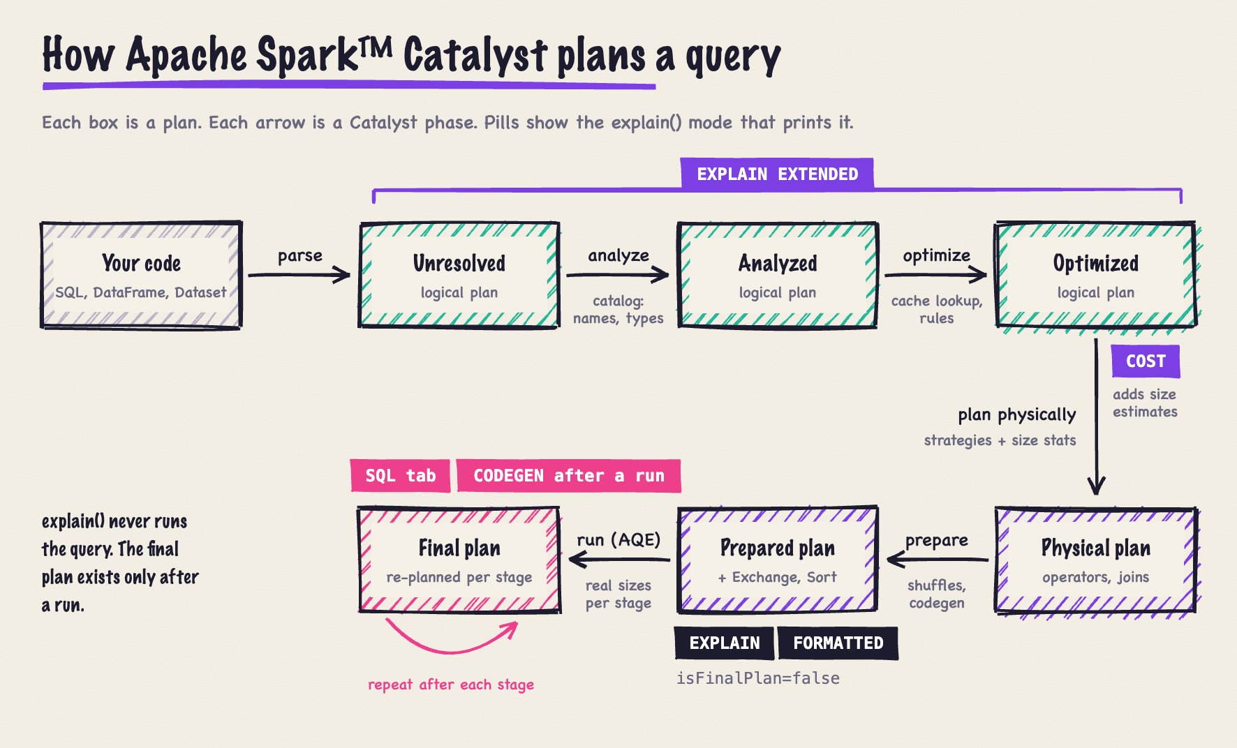
A query moves through seven stages:
- Parsing. The SQL parser or the DataFrame API builds an unresolved logical plan, where table and column names are still plain strings.
- Analysis. The analyzer resolves names against the catalog, gives every column a unique ID, checks types and inserts casts. A misspelled column fails here.
- Cache lookup. The cache manager swaps any subtree that matches a cached DataFrame for an
InMemoryRelation. - Logical optimization. Rule batches rewrite the plan into an equivalent one that does less work.
- Physical planning. Strategies turn logical operators into physical ones, for example a
Joininto aBroadcastHashJoinorSortMergeJoin. Spark takes the first plan its strategies produce, so size statistics mostly matter for join selection. - Preparation.
EnsureRequirementsinserts anExchange(a shuffle) and aSortwherever an operator needs its input partitioned or ordered differently.CollapseCodegenStagesfuses chains of operators into whole-stage code generation, Java that Spark compiles at runtime. - Adaptive execution. Adaptive query execution (AQE), on by default since Spark 3.2, splits the plan into query stages at each
Exchangeand re-optimizes the rest of the plan using each finished stage’s real output size.
A query to follow through every stage
The example uses two tables: 2 million customers, 5% of them enterprise accounts, and 20 million orders in 61 daily partitions. This builds them:
from datetime import date
from pyspark.sql import SparkSession, functions as F

spark = (SparkSession.builder.master("local[8]")
         .appName("catalyst-demo")
         .config("spark.sql.shuffle.partitions", "8")
         .getOrCreate())

countries = F.array(*[F.lit(c) for c in ["US", "DE", "GB", "IN", "FR",
                                         "BR", "JP", "CA", "AU", "NL"]])
customers = (
    spark.range(1, 2_000_001).withColumnRenamed("id", "customer_id")
    .withColumn("name", F.format_string("Customer %07d", "customer_id"))
    .withColumn("email",
                F.format_string("user%d@example.com", "customer_id"))
    .withColumn("segment",
                F.when(F.col("customer_id") % 20 == 0, "enterprise")
                .otherwise("consumer"))
    .withColumn("country", countries[F.abs(F.hash("customer_id")) % 10])
)
customers.write.saveAsTable("customers")

orders = (
    spark.range(1, 20_000_001).withColumnRenamed("id", "order_id")
    .withColumn("customer_id",
                (F.abs(F.hash("order_id")) % 2_000_000 + 1).cast("long"))
    .withColumn("status",
                F.when(F.rand(1) < 0.6, "shipped").otherwise("pending"))
    .withColumn("amount", (F.rand(2) * 500 + 5).cast("decimal(10,2)"))
    .withColumn("order_date",
                F.date_add(F.lit(date(2026, 9, 1)),
                           (F.col("order_id") % 61).cast("int")))
)
orders.write.partitionBy("order_date").saveAsTable("orders")
The query is a join plus an aggregation: revenue from shipped October orders placed by enterprise customers, by country. In PySpark:
orders = spark.table("orders")
customers = spark.table("customers")

revenue_by_country = (
    orders.join(customers, "customer_id")
    .where((F.col("order_date") >= "2026-10-01")
           & (F.col("status") == "shipped")
           & (F.col("segment") == "enterprise"))
    .groupBy("country")
    .agg(F.count("*").alias("orders"), F.sum("amount").alias("revenue"))
    .orderBy(F.desc("revenue"))
)
revenue_by_country.explain()
And in SQL:
EXPLAIN
SELECT c.country, count(*) AS orders, sum(o.amount) AS revenue
FROM orders o
JOIN customers c ON o.customer_id = c.customer_id
WHERE o.order_date >= '2026-10-01'
  AND o.status = 'shipped'
  AND c.segment = 'enterprise'
GROUP BY c.country
ORDER BY revenue DESC
Both versions filter after the join. Catalyst moves the filters below it, as the optimized plan shows next.
Logical plans: Parsed, analyzed and optimized
EXPLAIN EXTENDED prints three logical plans before the physical one. We use the SQL form here because the DataFrame API analyzes each step as you write it, so its parsed plan is already mostly resolved.
== Parsed Logical Plan ==
'Sort ['revenue DESC NULLS LAST], true
+- 'Aggregate ['c.country], ['c.country, 'count(1) AS orders#62, 'sum('o.amount) AS revenue#63]
   +- 'Filter ((('o.order_date >= 2026-10-01) AND ('o.status = shipped)) AND ('c.segment = enterprise))
      +- 'Join Inner, ('o.customer_id = 'c.customer_id)
         :- 'SubqueryAlias o
         :  +- 'UnresolvedRelation [orders], [], false
         +- 'SubqueryAlias c
            +- 'UnresolvedRelation [customers], [], false

== Analyzed Logical Plan ==
country: string, orders: bigint, revenue: decimal(20,2)
Sort [revenue#63 DESC NULLS LAST], true
+- Aggregate [country#21], [country#21, count(1) AS orders#62L, sum(amount#25) AS revenue#63]
   +- Filter (((order_date#26 >= cast(2026-10-01 as date)) AND (status#24 = shipped)) AND (segment#20 = enterprise))
      +- Join Inner, (customer_id#23L = customer_id#17L)
         :- SubqueryAlias o
         :  +- SubqueryAlias spark_catalog.default.orders
         :     +- Relation spark_catalog.default.orders[order_id#22L,customer_id#23L,status#24,amount#25,order_date#26] parquet
         +- SubqueryAlias c
            +- SubqueryAlias spark_catalog.default.customers
               +- Relation spark_catalog.default.customers[customer_id#17L,name#18,email#19,segment#20,country#21] parquet

== Optimized Logical Plan ==
Sort [revenue#63 DESC NULLS LAST], true
+- Aggregate [country#21], [country#21, count(1) AS orders#62L, sum(amount#25) AS revenue#63]
   +- Project [amount#25, country#21]
      +- Join Inner, (customer_id#23L = customer_id#17L)
         :- Project [customer_id#23L, amount#25]
         :  +- Filter ((((isnotnull(order_date#26) AND isnotnull(status#24)) AND (order_date#26 >= 2026-10-01)) AND (status#24 = shipped)) AND isnotnull(customer_id#23L))
         :     +- Relation spark_catalog.default.orders[order_id#22L,customer_id#23L,status#24,amount#25,order_date#26] parquet
         +- Project [customer_id#17L, country#21]
            +- Filter ((isnotnull(segment#20) AND (segment#20 = enterprise)) AND isnotnull(customer_id#17L))
               +- Relation spark_catalog.default.customers[customer_id#17L,name#18,email#19,segment#20,country#21] parquet
In the parsed plan, a leading apostrophe marks anything unresolved, such as 'UnresolvedRelation [orders] and 'c.country. The analyzed plan binds those names to catalog tables and gives every column an ID, so the two join keys become customer_id#23L (orders) and customer_id#17L (customers); the L marks a bigint. Because order_date is a date, the analyzer also wrapped the string literal in cast(2026-10-01 as date).
Optimization rules: What Catalyst rewrote
Comparing the analyzed and optimized plans shows the rule-based rewrites:
- Predicate pushdown (
PushDownPredicates): theFilterabove the join became one filter per side, so each table is filtered before the join. - Column pruning (
ColumnPruning): newProjectnodes keep only the two columns each side needs. - Constant folding (
ConstantFolding):cast(2026-10-01 as date)was evaluated at planning time and became the literal2026-10-01. - Combining and inferring filters (
CombineFilters,InferFiltersFromConstraints): conditions on one table merged into a singleFilter, and Catalyst addedisnotnull(customer_id)to both sides, because a null key can’t match an inner join.
Other rules fire when the shape fits. InjectRuntimeFilter, for example, adds a runtime Bloom filter to the probe side of a join that scans more than 10 GB by default, which our orders table doesn’t.
These rewrites need no data. Choosing a join strategy does, and without statistics Spark only has file sizes. explain(mode="cost") shows the estimates Catalyst used:
== Optimized Logical Plan ==
Sort [revenue#30 DESC NULLS LAST], true, Statistics(sizeInBytes=591.7 TiB)
+- Aggregate [country#21], [...], Statistics(sizeInBytes=591.7 TiB)
   +- Project [amount#25, country#21], Statistics(sizeInBytes=409.6 TiB)
      +- Join Inner, (...), Statistics(sizeInBytes=591.7 TiB)
         :- Project [...], Statistics(sizeInBytes=56.6 MiB)
         :  +- Filter (...), Statistics(sizeInBytes=132.1 MiB)
         :     +- Relation ...orders[...] parquet, Statistics(sizeInBytes=132.1 MiB)
         +- Project [...], Statistics(sizeInBytes=10.5 MiB)
            +- Filter (...), Statistics(sizeInBytes=27.9 MiB)
               +- Relation ...customers[...] parquet, Statistics(sizeInBytes=27.9 MiB)
Without column statistics, Spark can’t tell how selective segment = 'enterprise' is, so the customers Filter keeps the table’s 27.9 MiB estimate. The Project scales it by column width to 10.5 MiB, just over the 10 MB default for spark.sql.autoBroadcastJoinThreshold. Catalyst won’t broadcast customers, although only 100,000 rows survive the filter. The 591.7 TiB join estimate shows the same lack of row counts.
Cost-based optimization (CBO) fills that gap. After ANALYZE TABLE customers COMPUTE STATISTICS FOR COLUMNS customer_id, segment and with spark.sql.cbo.enabled set to true (it’s off by default), Catalyst estimates row counts and filter selectivity, and can reorder joins when spark.sql.cbo.joinReorder.enabled is on. CBO has two weak spots. It assumes values are evenly distributed: our plan estimated rowCount=1.00E+6 enterprise customers, half of 2 million, because segment has two distinct values. The real count is 100,000. Histograms (spark.sql.statistics.histogram.enabled) correct skewed distributions, but in our run Spark built one for the numeric customer_id and none for the string segment. And statistics are a snapshot from the last ANALYZE TABLE, so they go stale as data changes.
Physical planning: How Catalyst picks operators
For an equi-join like ours, the JoinSelection strategy checks these options in order:
- Broadcast hash join, if a hint asks for it or one side’s estimated size is at most
spark.sql.autoBroadcastJoinThreshold(10 MB). - Shuffled hash join, if
spark.sql.join.preferSortMergeJoinisfalse(it’strueby default) and one side is small enough to hash in each partition. - Sort-merge join otherwise, as long as the join keys can be sorted.
Joins without an equality condition fall back to BroadcastNestedLoopJoin or CartesianProduct. At 10.5 MiB, customers missed the first option, so the plan uses a sort-merge join.
A sort-merge join needs both inputs hash-partitioned on customer_id and sorted, so EnsureRequirements added an Exchange hashpartitioning(customer_id, 8) and a Sort to each side. The final aggregation needs each country’s rows in one partition (Exchange hashpartitioning(country, 8)), and ORDER BY needs a total order (Exchange rangepartitioning). The ENSURE_REQUIREMENTS label marks shuffles the planner inserted. One you request with repartition() carries a label such as REPARTITION_BY_NUM.
Running explain(): Every mode and what it shows
explain() plans the query without running it and prints the Spark explain plan. PySpark’s DataFrame.explain() takes a mode argument (since Spark 3.0), and SQL has matching EXPLAIN keywords:
| Mode | PySpark | SQL | What it prints |
|---|---|---|---|
| simple | df.explain() |
EXPLAIN |
The physical plan only |
| extended | df.explain(True) or mode="extended" |
EXPLAIN EXTENDED |
Parsed, analyzed and optimized logical plans, then the physical plan |
| codegen | mode="codegen" |
EXPLAIN CODEGEN |
The physical plan and the generated Java for each codegen stage |
| cost | mode="cost" |
EXPLAIN COST |
The optimized logical plan with size and row estimates, then the physical plan |
| formatted | mode="formatted" |
EXPLAIN FORMATTED |
A numbered outline of the physical plan, then details for each node |
Formatted mode is the easiest to scan, because it moves long operator arguments out of the tree:
== Physical Plan ==
AdaptiveSparkPlan (18)
+- Sort (17)
   +- Exchange (16)
      +- HashAggregate (15)
         +- Exchange (14)
            +- HashAggregate (13)
               +- Project (12)
                  +- SortMergeJoin Inner (11)
                     :- Sort (5)
                     :  +- Exchange (4)
                     :     +- Project (3)
                     :        +- Filter (2)
                     :           +- Scan parquet spark_catalog.default.orders (1)
                     +- Sort (10)
                        +- Exchange (9)
                           +- Project (8)
                              +- Filter (7)
                                 +- Scan parquet spark_catalog.default.customers (6)

(1) Scan parquet spark_catalog.default.orders
Output [4]: [customer_id#23L, status#24, amount#25, order_date#26]
Batched: true
Location: InMemoryFileIndex [file:/warehouse/orders/order_date=2026-10-29, ... 30 entries]
PartitionFilters: [isnotnull(order_date#26), (order_date#26 >= 2026-10-01)]
PushedFilters: [IsNotNull(status), EqualTo(status,shipped), IsNotNull(customer_id)]
ReadSchema: struct<customer_id:bigint,status:string,amount:decimal(10,2)>
...
The numbers follow the data, from the scans (1, 6) to the root (18).
Codegen mode has a catch. With AQE on, Spark plans code generation for each query stage when it runs, so before execution EXPLAIN CODEGEN prints only Found 0 WholeStageCodegen subtrees. After an action, explain(mode="codegen") on the same DataFrame reported five subtrees. In the first, the scan, filter and projection are fused into one loop, and a failed predicate skips to the next row:
== Subtree 1 / 5 (maxMethodCodeSize:362; maxConstantPoolSize:170(0.26% used); numInnerClasses:0) ==
*(1) Project [customer_id#23L, amount#25]
+- *(1) Filter ((isnotnull(status#24) AND (status#24 = shipped)) AND isnotnull(customer_id#23L))
   +- *(1) ColumnarToRow
      +- FileScan parquet spark_catalog.default.orders[...]

Generated code:
...
/* 044 */           boolean filter_value_2 = !columnartorow_isNull_1;
/* 045 */           if (!filter_value_2) continue;
/* 046 */
/* 047 */           boolean filter_value_3 = false;
/* 048 */           filter_value_3 = columnartorow_value_1.binaryEquals(((UTF8String) references[3] /* literal */));
/* 049 */           if (!filter_value_3) continue;
Reading a physical plan bottom-up
Here is the plain explain() output for revenue_by_country:
== Physical Plan ==
AdaptiveSparkPlan isFinalPlan=false
+- Sort [revenue#30 DESC NULLS LAST], true, 0
   +- Exchange rangepartitioning(revenue#30 DESC NULLS LAST, 8), ENSURE_REQUIREMENTS, [plan_id=110]
      +- HashAggregate(keys=[country#21], functions=[count(1), sum(amount#25)])
         +- Exchange hashpartitioning(country#21, 8), ENSURE_REQUIREMENTS, [plan_id=107]
            +- HashAggregate(keys=[country#21], functions=[partial_count(1), partial_sum(amount#25)])
               +- Project [amount#25, country#21]
                  +- SortMergeJoin [customer_id#23L], [customer_id#17L], Inner
                     :- Sort [customer_id#23L ASC NULLS FIRST], false, 0
                     :  +- Exchange hashpartitioning(customer_id#23L, 8), ENSURE_REQUIREMENTS, [plan_id=99]
                     :     +- Project [customer_id#23L, amount#25]
                     :        +- Filter ((isnotnull(status#24) AND (status#24 = shipped)) AND isnotnull(customer_id#23L))
                     :           +- FileScan parquet spark_catalog.default.orders[customer_id#23L,status#24,amount#25,order_date#26] Batched: true, DataFilters: [isnotnull(status#24), (status#24 = shipped), isnotnull(customer_id#23L)], Format: Parquet, Location: InMemoryFileIndex(31 paths)[file:/warehouse/..., PartitionFilters: [isnotnull(order_date#26), (order_date#26 >= 2026-10-01)], PushedFilters: [IsNotNull(status), EqualTo(status,shipped), IsNotNull(customer_id)], ReadSchema: struct<customer_id:bigint,status:string,amount:decimal(10,2)>
                     +- Sort [customer_id#17L ASC NULLS FIRST], false, 0
                        +- Exchange hashpartitioning(customer_id#17L, 8), ENSURE_REQUIREMENTS, [plan_id=100]
                           +- Project [customer_id#17L, country#21]
                              +- Filter ((isnotnull(segment#20) AND (segment#20 = enterprise)) AND isnotnull(customer_id#17L))
                                 +- FileScan parquet spark_catalog.default.customers[customer_id#17L,segment#20,country#21] Batched: true, DataFilters: [isnotnull(segment#20), (segment#20 = enterprise), isnotnull(customer_id#17L)], Format: Parquet, Location: InMemoryFileIndex(1 paths)[file:/warehouse/..., PartitionFilters: [], PushedFilters: [IsNotNull(segment), EqualTo(segment,enterprise), IsNotNull(customer_id)], ReadSchema: struct<customer_id:bigint,segment:string,country:string>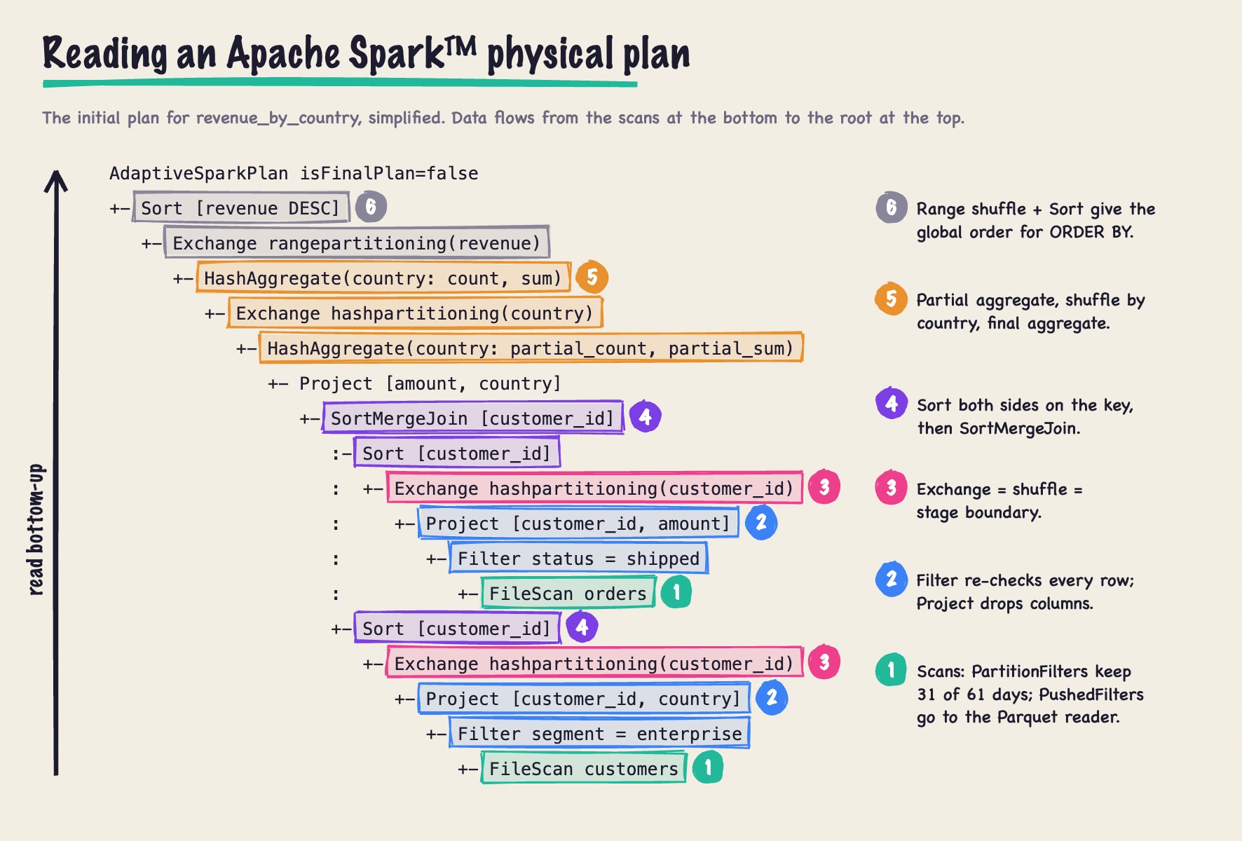
Spark prints the root first, but data flows up from the leaves, so start at the bottom. +- introduces a node’s last child and :- an earlier one, which is how the two sides of the join appear as separate branches.
- Scans.
PartitionFiltersshows partition pruning:InMemoryFileIndex(31 paths)means Spark reads 31 of the 61 daily partitions.PushedFilterslists the conditions handed to the Apache Parquet™ reader, which uses row-group statistics to skip data that can’t match.ReadSchemashows column pruning reaching the files: three columns are read from Parquet, andorder_datecomes from the directory name. - Filter and Project. Pushed filters only skip row groups, so the
Filterstill checks every row.Projectdrops unused columns. - Exchange. Each
Exchangeis a shuffle and a stage boundary. This plan has four: two for the join, one for the aggregation and one for the sort. - Join.
Sortorders each shuffled side bycustomer_id, andSortMergeJoinmerges the two sorted inputs. - Aggregation. The lower
HashAggregatecomputespartial_countandpartial_sumbefore the shuffle, so only one row per country per partition crosses the network. The upper one combines them. - Sort and root.
Exchange rangepartitioningandSortproduce the global order.AdaptiveSparkPlan isFinalPlan=falsemeans AQE may still change everything below it.
Plans that have run, or were planned with AQE off, also show codegen markers. *(3) means an operator belongs to whole-stage codegen stage 3, and operators sharing a number run as one generated function. With AQE off, this plan prints *(1) through *(7).
Operators worth recognizing
| Operator | What it does | What to check |
|---|---|---|
FileScan / Scan parquet |
Reads files | PartitionFilters, PushedFilters, ReadSchema |
HashAggregate |
Groups rows in a hash map; partial_ functions run before the shuffle |
Whether a partial aggregate exists below the Exchange |
Exchange |
Shuffles rows by hash, by range or to one partition | How many there are and which keys they use |
BroadcastExchange |
Collects one side and ships it to every executor | Its size, since it passes through the driver |
BroadcastHashJoin, SortMergeJoin, ShuffledHashJoin |
Equi-joins | Which strategy Spark picked, and why |
BroadcastNestedLoopJoin |
Joins without an equality condition | Large inputs, since it compares every pair |
TakeOrderedAndProject |
ORDER BY with LIMIT, without a global sort |
Present when you expected a top N |
Expand |
Duplicates rows for ROLLUP, CUBE and GROUPING SETS |
Row counts multiplied by the number of grouping sets (example) |
AQEShuffleRead |
AQE’s shuffle reader: coalesced, local or skew-split |
Present only in executed plans |
Join strategies in the plan
The join operator tells you how much data moved. BroadcastHashJoin ships the small side to every executor and streams the large side through it without a shuffle; BuildRight or BuildLeft names the broadcast side. SortMergeJoin shuffles and sorts both sides, the most expensive option but one that works at any size. ShuffledHashJoin shuffles both sides and hashes the smaller one per partition, skipping the sort (see shuffle hash join vs. sort-merge join).
To see why Spark picked a strategy, compare the smaller side’s cost-mode estimate with spark.sql.autoBroadcastJoinThreshold. Ours missed by 0.5 MiB. A join hint overrides the estimate: F.broadcast(customers) in PySpark or /*+ BROADCAST(c) */ in SQL. When the two sides carry different hints, Spark prefers BROADCAST, then MERGE, SHUFFLE_HASH and SHUFFLE_REPLICATE_NL. Hints aren’t guaranteed; Spark can’t broadcast the preserved side of an outer join, for example. With the hint, the orders side loses its Exchange and Sort:
+- BroadcastHashJoin [customer_id#23L], [customer_id#17L], Inner, BuildRight, false, false
   :- Project [customer_id#23L, amount#25]
   :  +- Filter ((isnotnull(status#24) AND (status#24 = shipped)) AND isnotnull(customer_id#23L))
   :     +- FileScan parquet spark_catalog.default.orders[...]
   +- BroadcastExchange HashedRelationBroadcastMode(List(input[0, bigint, true]),false), [plan_id=687]
      +- Project [customer_id#17L, country#21]
         +- Filter ((isnotnull(segment#20) AND (segment#20 = enterprise)) AND isnotnull(customer_id#17L))
            +- FileScan parquet spark_catalog.default.customers[...]
Adaptive query execution: Where the final plan lives
isFinalPlan=false means explain() printed the plan AQE started from. As each query stage finishes, AQE re-plans the rest using the stage’s real output size. It can coalesce small shuffle partitions, switch a sort-merge join to a broadcast join and split skewed partitions, often the fix for data skew.
To see the plan that ran, call explain() on the same DataFrame after an action:
AdaptiveSparkPlan isFinalPlan=true
+- == Final Plan ==
   ResultQueryStage 5
   +- *(5) Sort [revenue#30 DESC NULLS LAST], true, 0
      +- AQEShuffleRead coalesced
         +- ShuffleQueryStage 4
            +- Exchange rangepartitioning(revenue#30 DESC NULLS LAST, 8), ENSURE_REQUIREMENTS, [plan_id=632]
               +- *(4) HashAggregate(keys=[country#21], functions=[count(1), sum(amount#25)])
                  +- AQEShuffleRead coalesced
                     +- ShuffleQueryStage 3
                        +- Exchange hashpartitioning(country#21, 8), ENSURE_REQUIREMENTS, [plan_id=598]
                           +- *(3) HashAggregate(keys=[country#21], functions=[partial_count(1), partial_sum(amount#25)])
                              +- *(3) Project [amount#25, country#21]
                                 +- *(3) BroadcastHashJoin [customer_id#23L], [customer_id#17L], Inner, BuildRight, false, false
                                    :- AQEShuffleRead local
                                    :  +- ShuffleQueryStage 0
                                    :     +- Exchange hashpartitioning(customer_id#23L, 8), ENSURE_REQUIREMENTS, [plan_id=432]
                                    :        +- *(1) Project [customer_id#23L, amount#25]
                                    :           +- ...
                                    +- BroadcastQueryStage 2
                                       +- BroadcastExchange HashedRelationBroadcastMode(List(input[0, bigint, true]),false), [plan_id=516]
                                          +- AQEShuffleRead local
                                             +- ShuffleQueryStage 1
                                                +- Exchange hashpartitioning(customer_id#17L, 8), ENSURE_REQUIREMENTS, [plan_id=453]
                                                   +- *(2) Project [customer_id#17L, country#21]
                                                      +- ...
+- == Initial Plan ==
   ...
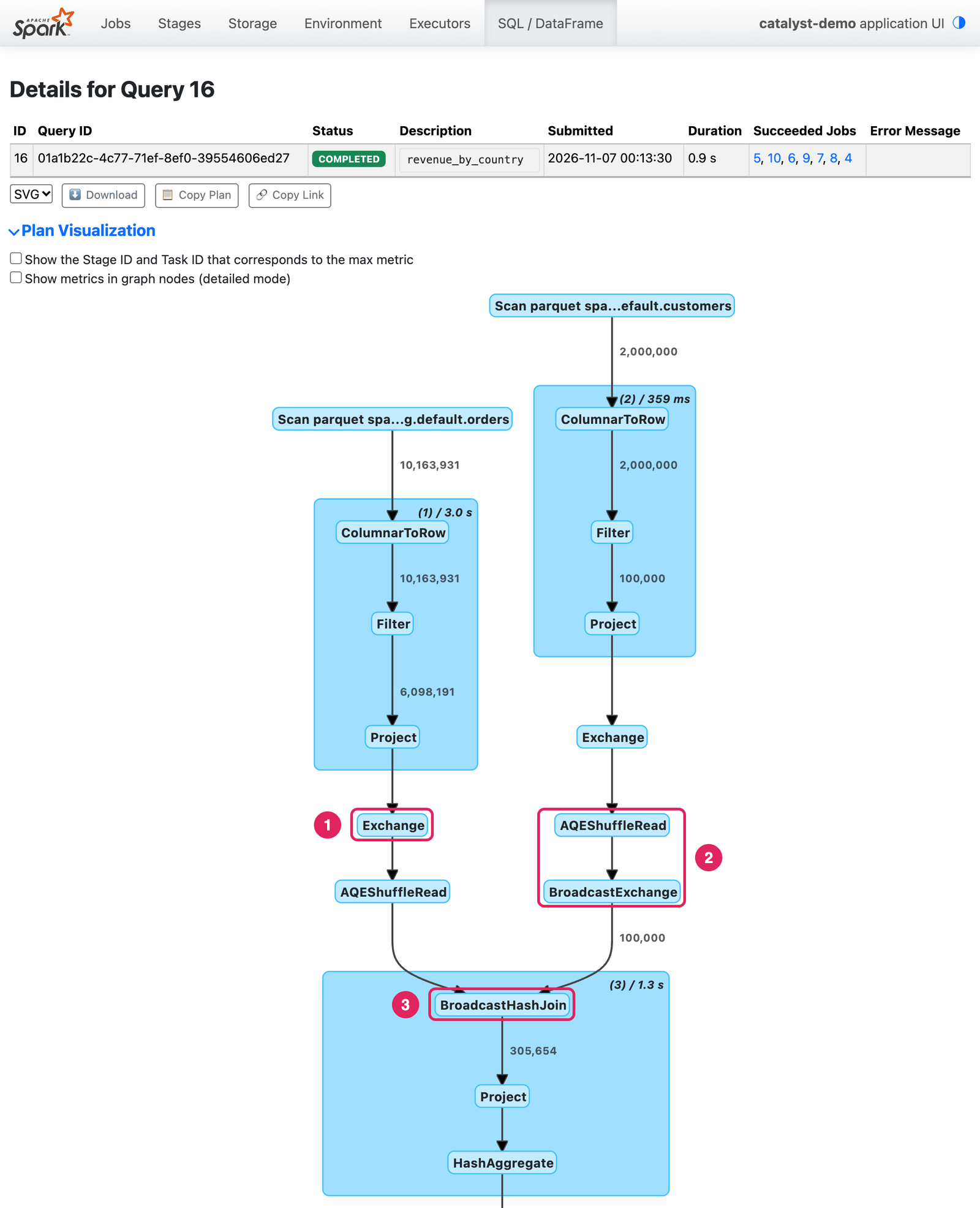
Once the customers stage finished, AQE measured 100,000 rows, under the broadcast threshold, and replaced the sort-merge join with a broadcast hash join. AQEShuffleRead coalesced means it merged small shuffle partitions. The orders side was still shuffled: ShuffleQueryStage 0 ran before AQE could re-plan, and AQEShuffleRead local just reads that output locally. The Spark docs call this conversion better than continuing the sort-merge join, but less efficient than planning a broadcast from the start.
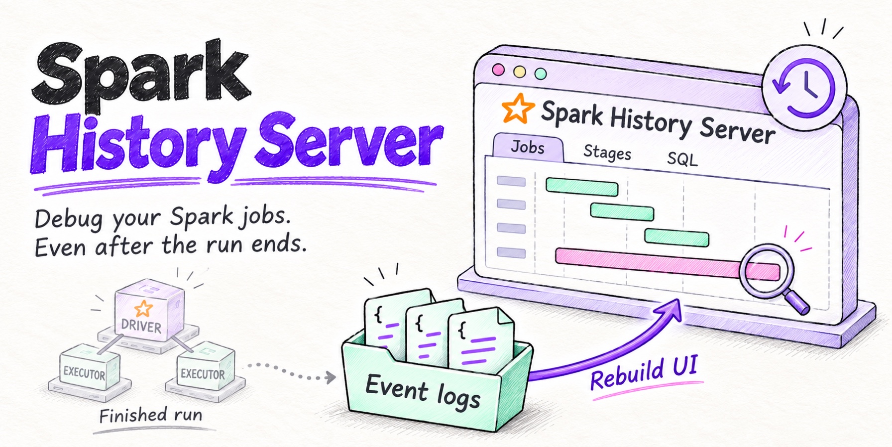
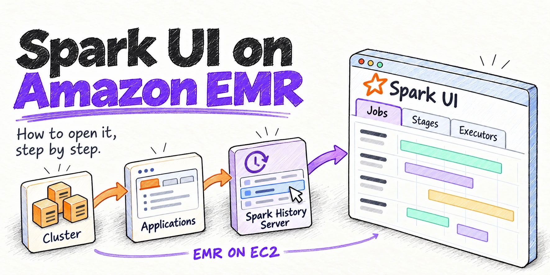
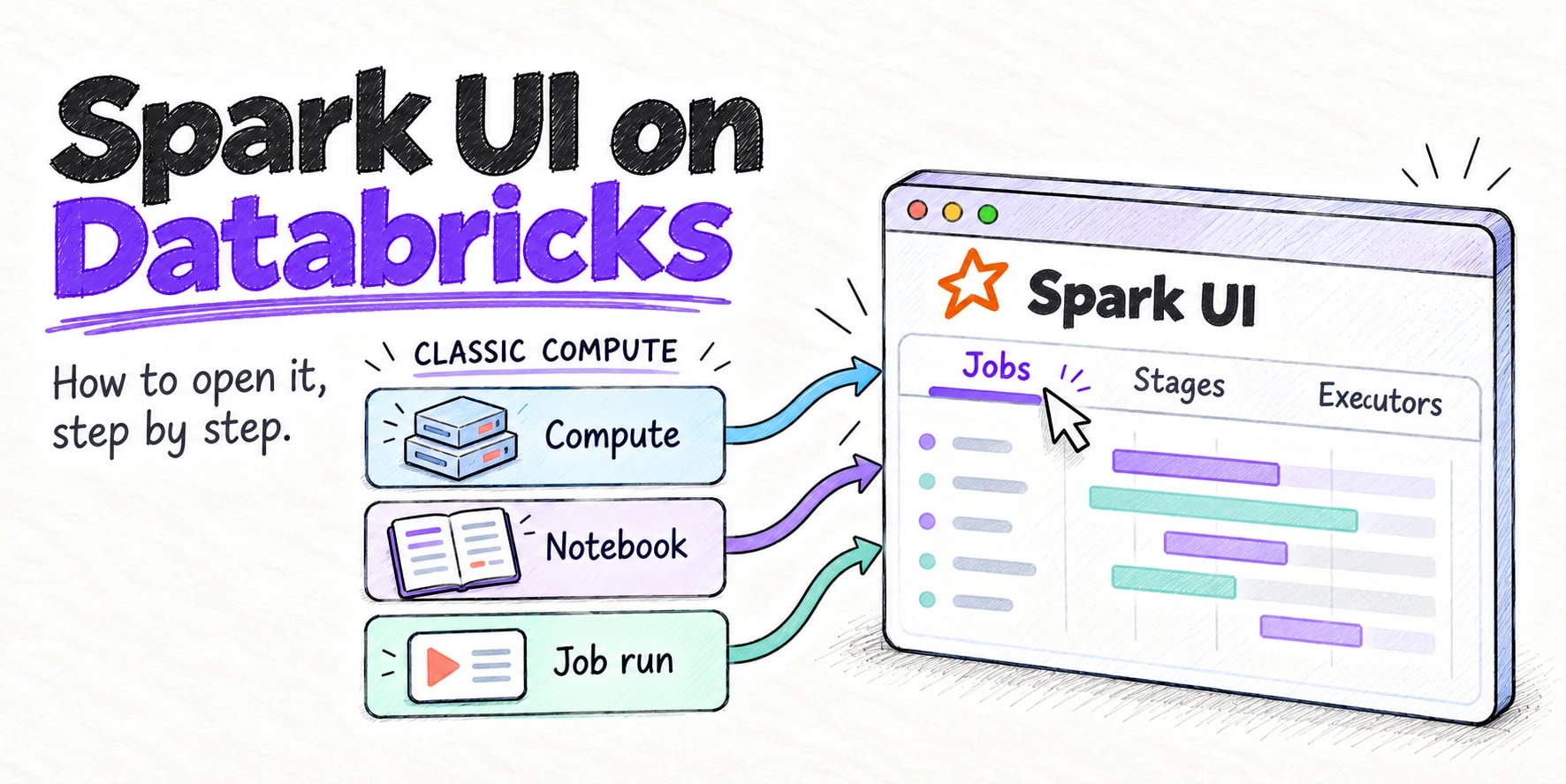
The Spark UI has the final plan for every query. Open the SQL / DataFrame tab and click a query to see its plan graph with row counts on each edge; Plan Details below it shows the text. For completed applications, the Spark History Server serves the same page, as covered in our guides to the Spark UI on Amazon EMR and Databricks.
Using the plan to debug slow queries
Most slow queries show up as one of a few patterns in the plan. Our Spark performance tuning guide covers the wider picture, including bad join strategies.
A sort-merge join where you expected a broadcast. Look for SortMergeJoin with an Exchange and a Sort under each side, then check the smaller side’s estimate in cost mode. If it’s wrong, as ours was, use a broadcast hint, raise spark.sql.autoBroadcastJoinThreshold slightly, or collect statistics. Relying on AQE still costs a shuffle: in our run it shuffled 6,098,191 order rows that the hint avoided.
Filters that never reach the scan. Compare DataFilters with PushedFilters. Rewriting status = 'shipped' as lower(status) = 'shipped' left this on the orders scan:
DataFilters: [isnotnull(status#24), (lower(status#24) = shipped)], ... PushedFilters: [IsNotNull(status)]Parquet can’t evaluate lower(), so every row group is read and filtered in Spark. Compare the raw column, or normalize values at write time. Filters through a UDF are never pushed, and a filter on a column derived from the partition key, such as to_date(order_ts) on a table partitioned by order_date, can’t prune partitions.
More shuffles than the query needs. Count the Exchange nodes and name the reason for each. Spark reuses partitioning where it can: grouping by customer_id, name, email right after the join on customer_id needed no new Exchange, and orderBy(...).limit(10) became a TakeOrderedAndProject with no range shuffle. A repartition() or grouping on a different key adds one.
Stale or misleading statistics. DESCRIBE EXTENDED customers shows the statistics CBO uses (29228116 bytes, 2000000 rows for ours), a snapshot from the last ANALYZE TABLE. Compare a node’s cost-mode rowCount with number of output rows in the SQL tab. A 10x gap, like our 1,000,000 estimate against 100,000 rows, means the plan was built on bad numbers. Re-run ANALYZE TABLE after large loads, and leave CBO off for tables without maintained statistics.
If you run Spark on Quanton, the Spark engine from Onehouse available on its own at quanton.dev, its free AI Spark Engineer sits in the Spark UI with the job’s SQL plans in context and can explain why a join wasn’t broadcast. Quanton can be used without the Onehouse platform, and you can create an account to try it.
FAQs
What is the Catalyst optimizer in Spark?
Catalyst is Spark SQL’s query optimizer. It turns SQL, DataFrame and Dataset code into a logical plan, applies rewrites such as predicate pushdown, column pruning and constant folding, picks physical operators and join strategies using size statistics, and generates Java code for groups of operators.
What is the difference between explain() and explain(True)?
explain() prints only the physical plan. explain(True), the same as explain(mode="extended") or EXPLAIN EXTENDED, also prints the parsed, analyzed and optimized logical plans, which show how Spark resolved names and which optimization rules changed the query.
Why does explain() show AdaptiveSparkPlan isFinalPlan=false?
Adaptive query execution is on, and explain() printed the initial plan before anything ran. AQE re-optimizes the plan as stages complete, so joins and partition counts can change. Call explain() again after an action, or open the query in the Spark UI SQL tab, to see the final plan.
Does the Spark Catalyst optimizer use cost-based optimization?
Partly. Catalyst always uses size estimates to choose join strategies, but full cost-based optimization, with row counts, filter selectivity and join reordering, needs spark.sql.cbo.enabled=true and statistics from ANALYZE TABLE ... COMPUTE STATISTICS FOR COLUMNS. Without them, Spark estimates from file sizes and column widths.